Production and Profit
Jennifer and Jason’s tomato farm will maximize its profit by producing bushels of tomatoes up to the point at which marginal revenue equals marginal cost. We know this from the producer’s optimal output rule introduced in Module 53—profit is maximized by producing the quantity at which the marginal revenue of the last unit produced is equal to its marginal cost. Always remember, MR = MC at the optimal quantity of output. This will be true for any profit-maximizing firm in any market structure.
We can review how to apply the optimal output rule with the help of Table 58.1, which provides various short-run cost measures for Jennifer and Jason’s farm. The second column contains the farm’s variable cost, and the third column shows its total cost based on the assumption that the farm incurs a fixed cost of $14. The fourth column shows the farm’s marginal cost. Notice that, in this example, the marginal cost initially falls as output rises but then begins to increase, so that the marginal cost curve has the familiar “swoosh” shape.
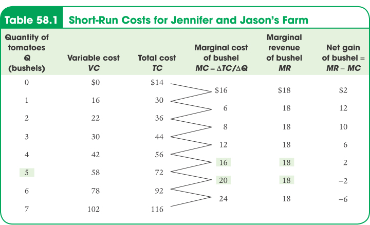
The fifth column contains the farm’s marginal revenue, which has an important feature: Jennifer and Jason’s marginal revenue is constant at $18 for every output level. The sixth and final column shows the calculation of the net gain per bushel of tomatoes, which is equal to the marginal revenue minus the marginal cost—or, equivalently in this case, the market price minus the marginal cost. As you can see, it is positive for the 1st through 5th bushels; producing each of these bushels raises Jennifer and Jason’s profit. For the 6th bushel, however, net gain is negative: producing it would decrease, not increase, profit. So 5 bushels are Jennifer and Jason’s profit-maximizing output; it is the level of output at which the marginal cost rises from a level below the market price to a level above the market price, passing through the market price of $18 along the way.

Anthony-Masterson/Digital Vision/Getty Images
The price-taking firm’s optimal output rule says that a price-taking firm’s profit is maximized by producing the quantity of output at which the market price is equal to the marginal cost of the last unit produced.
This example illustrates an application of the optimal output rule to the particular case of a price-taking firm—the price-taking firm’s optimal output rule: price equals marginal cost at the price-taking firm’s optimal quantity of output. That is, a price-taking firm’s profit is maximized by producing the quantity of output at which the market price is equal to the marginal cost of the last unit produced. Why? Because in the case of a price-taking firm, the marginal revenue is equal to the market price. A price-taking firm cannot influence the market price by its actions. It always takes the market price as given because it cannot lower the market price by selling more or raise the market price by selling less. So, for a price-taking firm, the additional revenue generated by producing one more unit is always the market price. We will need to keep this fact in mind in future modules, in which we will learn that in the three other market structures, firms are not price-takers. Therefore, the marginal revenue is not equal to the market price.
Figure 58.1 shows Jennifer and Jason’s profit-maximizing quantity of output. The figure shows the marginal cost curve, MC, drawn from the data in the fourth column of Table 58.1. We plot the marginal cost of increasing output from 1 to 2 bushels halfway between 1 and 2, and likewise for each incremental change. The horizontal line at $18 is Jennifer and Jason’s marginal revenue curve. Remember from Module 53 that whenever a firm is a price-taker, its marginal revenue curve is a horizontal line at the market price: it can sell as much as it likes at the market price. Regardless of whether it sells more or less, the market price is unaffected. In effect, the individual firm faces a horizontal, perfectly elastic demand curve for its output—a demand curve that is equivalent to its marginal revenue curve. In fact, the horizontal line with the height of the market price represents the perfectly competitive firm’s demand, marginal revenue, and average revenue—the average amount of revenue taken in per unit—because price equals average revenue whenever every unit is sold for the same price. The marginal cost curve crosses the marginal revenue curve at point E. Sure enough, the quantity of output at E is 5 bushels.
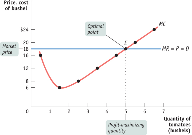
Figure 58.1: The Price-Taking Firm’s Profit-Maximizing Quantity of OutputAt the profit-maximizing quantity of output, the market price is equal to the marginal cost. It is located at the point where the marginal cost curve crosses the marginal revenue curve, which is a horizontal line at the market price and represents the firm’s demand curve. Here, the profit-maximizing point is at an output of 5 bushels of tomatoes, the output quantity at point E.
AP® Exam Tip
Notice that for a perfectly competitive firm, the horizontal line at the market price also represents the marginal revenue curve and the demand curve. Be prepared to draw and label this line for the AP® exam.
Does this mean that the price-taking firm’s production decision can be entirely summed up as “produce up to the point where the marginal cost of production is equal to the price”? No, not quite. Before applying the principle of marginal analysis to determine how much to produce, a potential producer must as a first step answer an “either–or” question: should it produce at all? If the answer to that question is yes, it then proceeds to the second step—a “how much” decision: maximizing profit by choosing the quantity of output at which the marginal cost is equal to the price.
To understand why the first step in the production decision involves an “either–or” question, we need to ask how we determine whether it is profitable or unprofitable to produce at all. In the next module we’ll see that unprofitable firms shut down in the long run, but tolerate losses in the short run up to a certain point.
When Is Production Profitable?
Remember from Module 52 that firms make their production decisions with the goal of maximizing economic profit—a measure based on the opportunity cost of resources used by the firm. In the calculation of economic profit, a firm’s total cost incorporates the implicit cost—the benefits forgone in the next best use of the firm’s resources—as well as the explicit cost in the form of actual cash outlays. In contrast, accounting profit is profit calculated using only the explicit costs incurred by the firm. This means that economic profit incorporates all of the opportunity cost of resources owned by the firm and used in the production of output, while accounting profit does not. A firm may make positive accounting profit while making zero or even negative economic profit. It’s important to understand that a firm’s decisions of how much to produce and whether or not to stay in business should be based on economic profit, not accounting profit.

South12th Photography/Shutterstock
So we will assume, as usual, that the cost numbers given in Table 58.1 include all costs, implicit as well as explicit. What determines whether Jennifer and Jason’s farm earns a profit or generates a loss? This depends on the market price of tomatoes—specifically, whether the market price is more or less than the farm’s minimum average total cost.
In Table 58.2 we calculate the short-run average variable cost and the short-run average total cost for Jennifer and Jason’s farm. These are short-run values because we take the fixed cost as given. (We’ll turn to the effects of changing fixed cost shortly.) The short-run average total cost curve, ATC, is shown in Figure 58.2, along with the marginal cost curve, MC, from Figure 58.1. As you can see, average total cost is minimized at point C, corresponding to an output of 4 bushels—the minimum-cost output—and an average total cost of $14 per bushel.
Table 58.2Short-Run Average Costs for Jennifer and Jason’s Farm
| Quantity of tomatoes Q (bushels) |
Variable cost VC |
Total cost TC |
Short-run average variable cost of bushel AVC = VC/Q |
Short-run average total cost of bushel ATC = TC/Q |
| 1 |
$16.00 |
$30.00 |
$16.00 |
$30.00 |
| 2 |
22.00 |
36.00 |
11.00 |
18.00 |
| 3 |
30.00 |
44.00 |
10.00 |
14.67 |
| 4 |
42.00 |
56.00 |
10.50 |
14.00 |
| 5 |
58.00 |
72.00 |
11.60 |
14.40 |
| 6 |
78.00 |
92.00 |
13.00 |
15.33 |
| 7 |
102.00 |
116.00 |
14.57 |
16.57 |
Table 58.1: Table 58.2 Short-Run Average Costs for Jennifer and Jason’s Farm
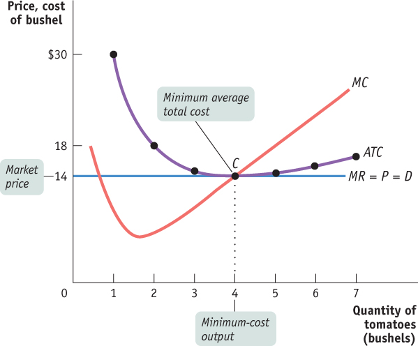
Figure 58.2: Costs and Production in the Short RunThis figure shows the marginal cost curve, MC, and the short-run average total cost curve, ATC. When the market price is $14, output will be 4 bushels of tomatoes (the minimum-cost output), represented by point C. The price of $14 is equal to the firm’s minimum average total cost, so at this price the firm breaks even.
To see how these curves can be used to decide whether production is profitable or unprofitable, recall that profit is equal to total revenue minus total cost, TR – TC. This means:
If the firm produces a quantity at which TR > TC, the firm is profitable.
If the firm produces a quantity at which TR = TC, the firm breaks even.
If the firm produces a quantity at which TR < TC, the firm incurs a loss.
We can also express this idea in terms of revenue and cost per unit of output. If we divide profit by the number of units of output, Q, we obtain the following expression for profit per unit of output:
(58-1) Profit/Q = TR/Q – TC/Q
TR/Q is average revenue, which is the market price. TC/Q is average total cost. So a firm is profitable if the market price for its product is more than the average total cost of the quantity the firm produces; a firm experiences losses if the market price is less than the average total cost of the quantity the firm produces. This means:
If the firm produces a quantity at which P > ATC, the firm is profitable.
If the firm produces a quantity at which P = ATC, the firm breaks even.
If the firm produces a quantity at which P < ATC, the firm incurs a loss.
In summary, in the short run a firm will maximize profit by producing the quantity of output at which MC = MR. A perfectly competitive firm is a price-taker, so it can sell as many units of output as it would like at the market price. This means that for a perfectly competitive firm it is always true that MR = P. The firm is profitable, or breaks even, as long as the market price is greater than, or equal to, the average total cost. In the next module, we develop the perfect competition model using graphs to analyze the firm’s level of profit.