Understanding Monopolistic Competition
AP® Exam Tip
In a monopolistically competitive industry there are many firms and low barriers to entry, as in a perfectly competitive industry. However, the sale of differentiated products gives the monopolistically competitive firms some monopoly power.
Suppose an industry is monopolistically competitive: it consists of many producers, all competing for the same consumers but offering differentiated products. How does such an industry behave?
As the term monopolistic competition suggests, this market structure combines some features typical of monopoly with others typical of perfect competition. Because each firm is offering a distinct product, it is in a way like a monopolist: it faces a downward-sloping demand curve and has some market power—the ability within limits to determine the price of its product. However, unlike a pure monopolist, a monopolistically competitive firm does face competition: the amount of its product it can sell depends on the prices and products offered by other firms in the industry.
The same, of course, is true of an oligopoly. In a monopolistically competitive industry, however, there are many producers, as opposed to the small number that defines an oligopoly. This means that the “puzzle” of oligopoly—whether firms will collude or behave noncooperatively—does not arise in the case of monopolistically competitive industries. True, if all the gas stations or all the restaurants in a town could agree—explicitly or tacitly—to raise prices, it would be in their mutual interest to do so. But such collusion is virtually impossible when the number of firms is large and, by implication, there are no barriers to entry. So in situations of monopolistic competition, we can safely assume that firms behave noncooperatively and ignore the potential for collusion.
Monopolistic Competition in the Short Run
We introduced the distinction between short-run and long-run equilibrium when we studied perfect competition. The short-run equilibrium of an industry takes the number of firms as given. The long-run equilibrium, by contrast, is reached only after enough time has elapsed for firms to enter or exit the industry. To analyze monopolistic competition, we focus first on the short run and then on how an industry moves from the short run to the long run.
Panels (a) and (b) of Figure 67.1 show two possible situations that a typical firm in a monopolistically competitive industry might face in the short run. In each case, the firm looks like any monopolist: it faces a downward-sloping demand curve, which implies a downward-sloping marginal revenue curve.
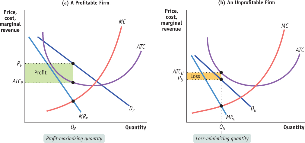
Figure 67.1: The Monopolistically Competitive Firm in the Short RunThe firm in panel (a) can be profitable for some output quantities: the quantities for which its average total cost curve, ATC, lies below its demand curve, DP. The profit-maximizing output quantity is QP, the output at which marginal revenue, MRP, is equal to marginal cost, MC. The firm charges price PP and earns a profit, represented by the area of the green shaded rectangle. The firm in panel (b), however, can never be profitable because its average total cost curve lies above its demand curve, DU, for every output quantity. The best that it can do if it produces at all is to produce quantity QU and charge price PU. This generates a loss, indicated by the area of the orange shaded rectangle. Any other output quantity results in a greater loss.
We assume that every firm has an upward-sloping marginal cost curve but that it also faces some fixed costs, so that its average total cost curve is U-shaped. This assumption doesn’t matter in the short run; but, as we’ll see shortly, it is crucial to understanding the long-run equilibrium.
AP® Exam Tip
Like a monopolist, a monopolistically competitive firm faces a downward-sloping demand curve and a marginal revenue curve that is below the demand curve. Unlike a monopolist, a monopolistically competitive firm will necessarily earn zero economic profit in the long run.
In each case the firm, in order to maximize profit, sets marginal revenue equal to marginal cost. So how do these two figures differ? In panel (a) the firm is profitable; in panel (b) it is unprofitable. (Recall that we are referring always to economic profit and not accounting profit—that is, a profit given that all factors of production are earning their opportunity costs.)
In panel (a) the firm faces the demand curve DP and the marginal revenue curve MRP. It produces the profit-maximizing output QP, the quantity at which marginal revenue is equal to marginal cost, and sells it at the price PP. This price is above the average total cost at this output, ATCP. The firm’s profit is indicated by the area of the shaded rectangle.
In panel (b) the firm faces the demand curve DU and the marginal revenue curve MRU. It chooses the quantity QU at which marginal revenue is equal to marginal cost. However, in this case the price PU is below the average total cost ATCU; so at this quantity the firm loses money. Its loss is equal to the area of the shaded rectangle. Since QU is the profit-maximizing quantity—which means, in this case, the loss-minimizing quantity—there is no way for a firm in this situation to make a profit. We can confirm this by noting that at any quantity of output, the average total cost curve in panel (b) lies above the demand curve DU. Because ATC > P at all quantities of output, this firm always suffers a loss.
As this comparison suggests, the key to whether a firm with market power is profitable or unprofitable in the short run lies in the relationship between its demand curve and its average total cost curve. In panel (a) the demand curve DP crosses the average total cost curve, meaning that some of the demand curve lies above the average total cost curve. So there are some price–quantity combinations available at which price is higher than average total cost, indicating that the firm can choose a quantity at which it makes positive profit.
In panel (b), by contrast, the demand curve DU does not cross the average total cost curve—it always lies below it. So the price corresponding to each quantity demanded is always less than the average total cost of producing that quantity. There is no quantity at which the firm can avoid losing money.
These figures, showing firms facing downward-sloping demand curves and their associated marginal revenue curves, look just like ordinary monopoly graphs. The “competition” aspect of monopolistic competition comes into play, however, when we move from the short run to the long run.
Monopolistic Competition in the Long Run
Obviously, an industry in which existing firms are losing money, like the one in panel (b) of Figure 67.1, is not in long-run equilibrium. When existing firms are losing money, some firms will exit the industry. The industry will not be in long-run equilibrium until the persistent losses have been eliminated by the exit of some firms.
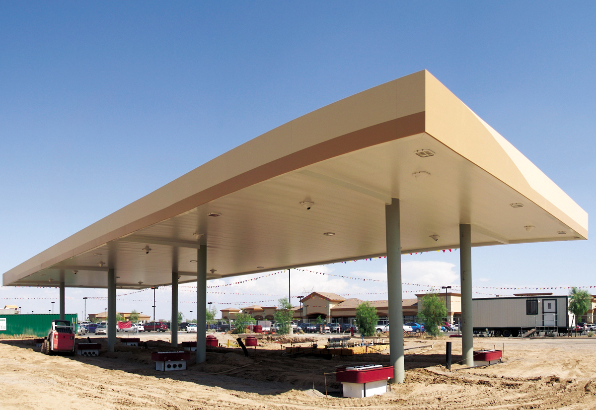
In the long-run, profit lures new firms to enter an industry.
Anton Foltin/Shutterstock
It may be less obvious that an industry in which existing firms are earning profits, like the one in panel (a) of Figure 67.1, is also not in long-run equilibrium. Given there is free entry into the industry, persistent profits earned by the existing firms will lead to the entry of additional producers. The industry will not be in long-run equilibrium until the persistent profits have been eliminated by the entry of new producers.
How will entry or exit by other firms affect the profit of a typical existing firm? Because the differentiated products offered by firms in a monopolistically competitive industry are available to the same set of customers, entry or exit by other firms will affect the demand curve facing every existing producer. If new gas stations open along a highway, each of the existing gas stations will no longer be able to sell as much gas as before at any given price. So, as illustrated in panel (a) of Figure 67.2, entry of additional producers into a monopolistically competitive industry will lead to a leftward shift of the demand curve and the marginal revenue curve facing a typical existing producer.
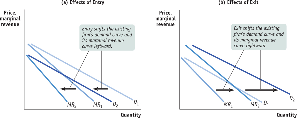
Figure 67.2: Entry and Exit Shift Existing Firms’ Demand Curves and Marginal Revenue CurvesEntry will occur in the long run when existing firms are profitable. In panel (a), entry causes each existing firm’s demand curve and marginal revenue curve to shift to the left. The firm receives a lower price for every unit it sells, and its profit falls. Entry will cease when firms make zero profit. Exit will occur in the long run when existing firms are unprofitable. In panel (b), exit from the industry shifts each remaining firm’s demand curve and marginal revenue curve to the right. The firm receives a higher price for every unit it sells, and profit rises. Exit will cease when the remaining firms make zero profit.
Conversely, suppose that some of the gas stations along the highway close. Then each of the remaining stations will be able to sell more gasoline at any given price. So as illustrated in panel (b), exit of firms from an industry leads to a rightward shift of the demand curve and marginal revenue curve facing a typical remaining producer.
In the long run, a monopolistically competitive industry ends up in zero-profit equilibrium: each firm makes zero profit at its profit-maximizing quantity.
The industry will be in long-run equilibrium when there is neither entry nor exit. This will occur only when every firm earns zero profit. So in the long run, a monopolistically competitive industry will end up in zero-profit equilibrium, in which firms just manage to cover their costs at their profit-maximizing output quantities.
We have seen that a firm facing a downward-sloping demand curve will earn positive profit if any part of that demand curve lies above its average total cost curve; it will incur a loss if its entire demand curve lies below its average total cost curve. So in zero-profit equilibrium, the firm must be in a borderline position between these two cases; its demand curve must just touch its average total cost curve. That is, the demand curve must be just tangent to the average total cost curve at the firm’s profit-maximizing output quantity—the output quantity at which marginal revenue equals marginal cost.
If this is not the case, the firm operating at its profit-maximizing quantity will find itself making either a profit or loss, as illustrated in the panels of Figure 67.1. But we also know that free entry and exit means that this cannot be a long-run equilibrium. Why? In the case of a profit, new firms will enter the industry, shifting the demand curve of every existing firm leftward until all profit is eliminated. In the case of a loss, some existing firms exit and so shift the demand curve of every remaining firm to the right until all losses are eliminated. All entry and exit ceases only when every existing firm makes zero profit at its profit-maximizing quantity of output.
Figure 67.3 shows a typical monopolistically competitive firm in such a zero-profit equilibrium. The firm produces QMC, the output at which MRMC = MC, and charges price PMC. At this price and quantity, represented by point Z, the demand curve is just tangent to its average total cost curve. The firm earns zero profit because price, PMC, is equal to average total cost, ATCMC.
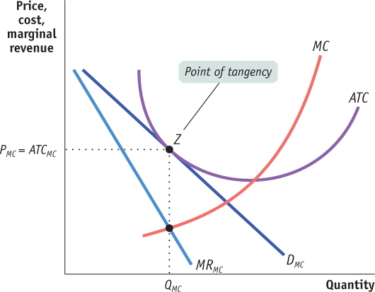
Figure 67.3: The Long-Run Zero-Profit EquilibriumIf existing firms are profitable, entry will occur and shift each existing firm’s demand curve leftward. If existing firms are unprofitable, each remaining firm’s demand curve shifts rightward as some firms exit the industry. Entry and exit will cease when every existing firm makes zero profit at its profit-maximizing quantity. So, in long-run zero-profit equilibrium, the demand curve of each firm is tangent to its average total cost curve at its profit-maximizing quantity: at the profit-maximizing quantity, QMC, price, PMC, equals average total cost, ATCMC. A monopolistically competitive firm is like a monopolist without monopoly profits.
The normal long-run condition of a monopolistically competitive industry, then, is that each producer is in the situation shown in Figure 67.3. Each producer acts like a monopolist, facing a downward-sloping demand curve and setting marginal cost equal to marginal revenue so as to maximize profit. But this is just enough to achieve zero economic profit. The producers in the industry are like monopolists without monopoly profit.
Hits and Flops
On the face of it, the movie business seems to meet the criteria for monopolistic competition. Movies compete for the same consumers; each movie is different from the others; new companies can and do enter the business. But where’s the zero-profit equilibrium? After all, some movies are enormously profitable.
The key is to realize that for every successful blockbuster, there are several flops—and that the movie studios don’t know in advance which will be which. (One observer of Hollywood summed up his conclusions as follows: “Nobody knows anything.”) By the time it becomes clear that a movie will be a flop, it’s too late to cancel it.
The difference between movie-making and the type of monopolistic competition we model in this section is that the fixed costs of making a movie are also sunk costs—once they’ve been incurred, they can’t be recovered.
Yet there is still, in a way, a zero-profit equilibrium. If movies on average were highly profitable, more studios would enter the industry and more movies would be made. If movies on average lost money, fewer movies would be made. In fact, as you might expect, the movie industry on average earns just about enough to cover the cost of production—that is, it earns roughly zero economic profit.
This kind of situation—in which firms earn zero profit on average but have a mixture of highly profitable hits and money-losing flops—can be found in other industries characterized by high up-front sunk costs. A notable example is the pharmaceutical industry, in which many research projects lead nowhere but a few lead to highly profitable drugs.

AP Photo/Nick Ut