If several alternative input combinations can be used to produce the optimal level of output, a profit-maximizing firm will select the input combination with the lowest cost. This process is known as cost minimization.

How does a firm determine the combination of inputs that maximizes profit? Let’s consider this question using an example.

Imagine you manage a grocery store chain and you need to decide the right combination of self-checkout stations and cashiers at a new store. Table 72.1 shows the alternative combinations of capital (self-checkout stations) and labor (cashiers) you can hire to check out customers shopping at the store. If the store puts in 20 self-checkout stations, you will need to hire 1 cashier to monitor every 5 stations for a total of 4 cashiers. However, trained cashiers are faster than customers at scanning goods, so the store could check out the same number of customers using 10 cashiers and only 10 self-checkout stations.

If you can check out the same number of customers using either of these combinations of capital and labor, how do you decide which combination of inputs to use? By finding the input combination that costs the least—the cost-minimizing input combination.

717

Assume that the cost to rent, operate, and maintain a self-checkout station for a month is $1,000 and hiring a cashier costs $1,600 per month. The cost of each input combination from Table 72.1 is shown below.

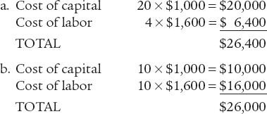
Clearly, your grocery store chain would choose the lower cost combination, combination b, and hire 10 cashiers and put 10 self-checkout stations in the new store.

When firms must choose among alternative combinations of inputs, they evaluate the cost of each combination and select the one that minimizes the cost of production. This can be done by calculating the total cost of each alternative combination of inputs, as shown in this example. However, because the number of possible combinations can be very large, it is more practical to use marginal analysis to find the cost-minimizing level of output—which brings us to the cost-minimization rule.

We already know that the additional output that results from employing an additional unit of an input is the marginal product (MP) of that input. Firms want to receive the highest possible marginal product from each dollar spent on inputs. To do this, firms adjust their combination of inputs until the marginal product per dollar is equal for all inputs. This is the cost-minimization rule. When the inputs are labor and capital, this amounts to equating the marginal product of labor (MPL) per dollar spent on wages to the marginal product of capital (MPK) per dollar spent to rent capital:

(72-1) MPL/Wage = MPK/Rental rate

To understand why cost minimization occurs when the marginal product per dollar is equal for all inputs, let’s start by looking at two counterexamples. Consider a situation in which the marginal product of labor per dollar is greater than the marginal product of capital per dollar. This situation is described by Equation 72-2:

(72-2) MPL/Wage > MPK/Rental rate

Suppose the marginal product of labor is 20 units and the marginal product of capital is 100 units. If the wage is $10 and the rental rate for capital is $100, then the marginal product per dollar will be 20/$10 = 2 units of output per dollar for labor and 100/$100 = 1 unit of output per dollar for capital. The firm is receiving 2 additional units of output for each dollar spent on labor and only 1 additional unit of output for each dollar spent on capital. In this case, the firm gets more additional output for its money by hiring labor, so it should hire more labor and rent less capital. Because of diminishing returns, as the firm hires more labor, the marginal product of labor falls and as it rents less capital, the marginal product of capital rises. The firm will continue to substitute labor for capital until the falling marginal product of labor per dollar meets the rising marginal product of capital per dollar and the two are equivalent. That is, the firm will adjust its quantities of capital and labor until the marginal product per dollar spent on each input is equal, as in Equation 72-1.

Next, consider a situation in which the marginal product of capital per dollar is greater than the marginal product of labor per dollar. This situation is described by Equation 72-3:

(72-3) MPL/Wage < MPK/Rental rate

718

Let’s continue with the assumption that the marginal product of labor for the last unit of labor hired is 20 units and the marginal product of capital for the last unit of capital rented is 100 units. If the wage is $10 and the rental rate for capital is $25, then the marginal product per dollar will be 20/$10 = 2 units of output per dollar for labor and 100/$25 = 4 units of output per dollar for capital. The firm is receiving 4 additional units of output for each dollar spent on capital and only 2 additional units of output for each dollar spent on labor. In this case, the firm gets more additional output for its money by renting capital, so it should rent more capital and hire less labor. Because of diminishing returns, as the firm rents more capital, the marginal product of capital falls, and as it hires less labor, the marginal product of labor rises. The firm will continue to rent more capital and hire less labor until the falling marginal product of capital per dollar meets the rising marginal product of labor per dollar to satisfy the cost-minimization rule. That is, the firm will adjust its quantities of capital and labor until the marginal product per dollar spent on each input is equal.

The cost-minimization rule is analogous to the optimal consumption rule (introduced in Module 51), which has consumers maximize their utility by choosing the combination of goods so that the marginal utility per dollar is equal for all goods.

So far in this section we have learned how factor markets determine the equilibrium price and quantity in the markets for land, labor, and capital and how firms determine the combination of inputs they will employ. But how well do these models of factor markets explain the distribution of factor incomes in our economy? In Module 70 we considered how the marginal productivity theory of income distribution explains the factor distribution of income. In the final module in this section we look at the distribution of income in labor markets and consider to what extent the marginal productivity theory of income distribution explains wage differences.