The Supply Curve
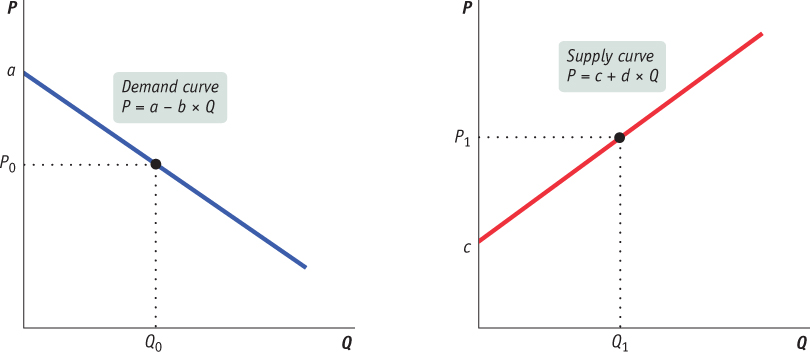
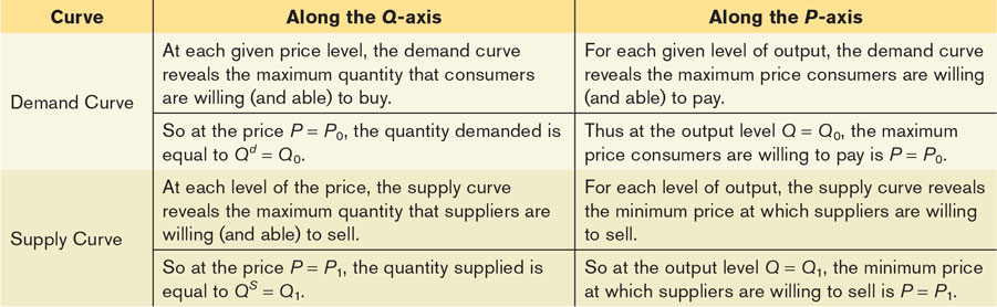
Usually, in the short run, other things equal, the supply curve is an upward sloping function of the price of the good or service being studied. For each level of output, the supply curve reveals the minimum price at which suppliers are willing to sell. Similarly, at each level of the price the supply curve reveals the maximum quantity that suppliers are willing to sell. In the case of linear expressions, a supply curve in its simplest form would be:
where P is the price, QS is the quantity, and c and d are positive constants.3 That d × QS is added to a constant tells us that as price rises, all else constant, a higher level of quantity is supplied and vice versa (the supply curve slopes upward). The d term describes how sensitive the price is to changes in the quantity supplied (i.e., the slope of the supply curve). If d takes on a larger value then the supply curve becomes relatively steeper—
Again, the simple appearance of Equation 3A-

with c expanded to include several factors multiplied by constants that are summarized in Table 3A-2. These factors are all multiplied by positive constants that, like d, describe how sensitive the supply curve is to change in those factors. The constant c0 picks up the impact of all other determinants of the supply of maple syrup that have been left out of the equation of the supply curve. Like the demand curve, if any of these values change, then the supply curve changes too. Figure 3A-2 examines a shift in the supply curve using algebra.
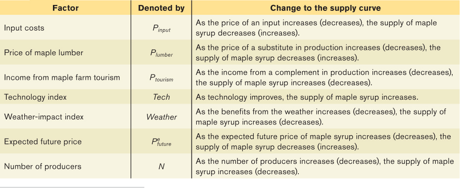
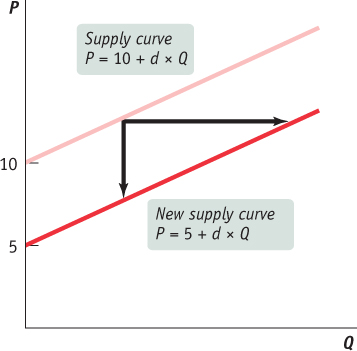
Note that if supply decreases (i.e., c increases), the supply curve shifts up (or to the left).
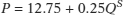
Suppose that, given a set of values for all the factors and constants, we get the following supply curve for maple syrup:
Before we use the demand and supply curves for maple syrup to find the equilibrium price and quantity, let’s look at Figure 3A-3, which provides a visual summary of the demand and supply curves. For a summary of how to interpret points along these curves, see Table 3A-3.