There is a lively market in used university and college textbooks. At the end of each term, some of the students who took a course decide that the money they can get by selling their used books is worth more to them than keeping the books. And some students who are taking the course next term prefer to buy a somewhat battered but cheaper used textbook than a new textbook at full price.

Textbook publishers and authors may not be happy about these transactions because they cut into sales of new books. But both the students who sell used books and those who buy them clearly benefit from the existence of the resale market. That is why many campus bookstores facilitate the trade in used textbooks, buying and selling them alongside the new books.

So, can we put a number on the benefit that used textbook buyers and sellers gain from these transactions? Can we answer the question “How much do the buyers and sellers of textbooks gain from the existence of the used book market?” Yes, we can.

Let’s start with the buyers. The key point, as we’ll see in a minute, is that the demand curve is derived from buyers’ tastes or preferences—and that those same preferences also determine how much they gain from the opportunity to buy used books.

Willingness to Pay and the Demand Curve A used book is not as good as a new book—it will be scuffed up and coffee-stained, may include someone else’s highlighting, and may not be completely up to date. How much this bothers you depends on your preferences. Some potential buyers would prefer to buy the used book even if it is only slightly cheaper than a new one; others would buy the used book only if it is considerably cheaper. Let’s define a potential buyer’s willingness to pay as the maximum price at which he or she would buy a good, in this case a used textbook. An individual won’t buy the book if it costs more than this amount but will be eager to do so if it costs less. If the price is just equal to an individual’s willingness to pay, he or she is indifferent to buying or not buying.

Table 3B-1 shows five potential buyers of a used book that costs $100 new, listed in order of their willingness to pay. At one extreme is Aleisha, who will buy a second-hand book even if the price is as high as $59. Brad is less willing to have a used book and will buy one only if the price is $45 or less. Claudia is willing to pay only $35; Darren, only $25. And Emiko, who really doesn’t like the idea of a used book, will buy one only if it costs no more than $10.

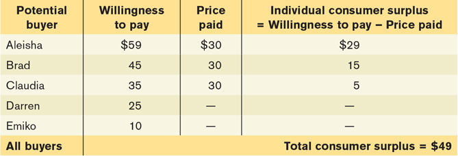
How many of these five students will actually buy a used book? It depends on the price. If the price of a used book is $55, only Aleisha will buy one; if the price is $40, Aleisha and Brad will both buy used books, and so on. So the information in the table also defines the demand schedule for used textbooks.

Willingness to Pay and Consumer Surplus Suppose that the campus bookstore makes used textbooks available at a price of $30. In that case Aleisha, Brad, and Claudia will buy used books. Do they gain from their purchases, and if so, how much?

The answer, also shown in Table 3B-1, is that each student who purchases a used book does achieve a net gain but that the amount of the gain differs among students.

Aleisha would have been willing to pay $59, so her net gain is $59 − $30 = $29. Brad would have been willing to pay $45, so his net gain is $45 − $30 = $15. Claudia would have been willing to pay $35, so her net gain is $35 − $30 = $5. Darren and Emiko, however, wouldn’t be willing to buy a used book at a price of $30, so they would neither gain nor lose.

The net gain that a buyer achieves from the purchase of a good is called that buyer’s individual consumer surplus. What we learn from this example is that whenever a buyer pays a price less than his or her willingness to pay, the buyer achieves some individual consumer surplus.

The sum of the individual consumer surpluses achieved by all the buyers of a good is known as the total consumer surplus achieved in the market. In Table 3B-1, the total consumer surplus is the sum of the individual consumer surpluses achieved by Aleisha, Brad, and Claudia: $29 + $15 + $5 = $49.

Economists use the term consumer surplus to refer to both individual and total consumer surplus. We will follow this practice; it will always be clear in context whether we are referring to the consumer surplus achieved by an individual or by all buyers.

Total consumer surplus can be represented graphically. As we saw in this chapter, we can use the demand schedule to derive the market demand curve shown in Figure 3B-1. Because we are considering only a small number of consumers, this curve doesn’t look like the smooth demand curves of this chapter, where markets contained hundreds or thousands of consumers. Instead, this demand curve is stepped, with alternating horizontal and vertical segments. Each horizontal segment—each step—corresponds to one potential buyer’s willingness to pay. Each step in that demand curve is one used book wide and represents one consumer. For example, the height of Aleisha’s step is $59, her willingness to pay. This step forms the top of a rectangle, with $30—the price she actually pays for a used book—forming the bottom. The area of Aleisha’s rectangle, ($59 − $30) × 1 = $29, is her consumer surplus from purchasing one used book at $30. So the individual consumer surplus Aleisha gains is the area of the dark blue rectangle shown in Figure 3B-1.

In addition to Aleisha, Brad and Claudia will also each buy a used book when the price is $30. Like Aleisha, they will benefit from their purchases, though not as much, because they each have a lower willingness to pay. Figure 3B-1 also shows the consumer surplus gained by Brad and Claudia; again, this can be measured by the areas of the appropriate rectangles. Darren and Emiko, because they do not buy used books at a price of $30, receive no consumer surplus.

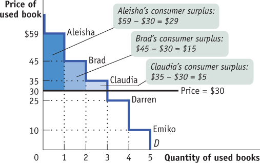
The total consumer surplus achieved in this market is the sum of the individual consumer surpluses received by Aleisha, Brad, and Claudia. So total consumer surplus is equal to the combined area of the three rectangles—the entire shaded area in Figure 3B-1. Another way to say this is that total consumer surplus is equal to the area below the demand curve but above the price.

This illustrates the following general principle: the total consumer surplus generated by purchases of a good at a given price is equal to the area below the demand curve but above that price. The same principle applies regardless of the number of consumers.

For large markets, this graphical representation of consumer surplus becomes extremely helpful. Consider, for example, the sales of tablet computers to millions of potential buyers. Each potential buyer has a maximum price that he or she is willing to pay. With so many potential buyers, the demand curve will be smooth, like the one shown in Figure 3B-2.

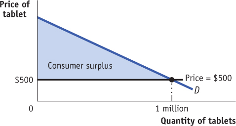
Suppose that at a price of $500, a total of 1 million tablets are purchased. How much do consumers gain from being able to buy those 1 million tablets? We could answer that question by calculating the consumer surplus of each individual buyer and then adding these numbers up to arrive at a total. But it is much easier just to look at Figure 3B-2 and use the fact that the total consumer surplus is equal to the shaded area. As in our original example, consumer surplus is equal to the area below the demand curve but above the price. (You can refresh your memory on how to calculate the area of a right triangle by reviewing Appendix 2A.)