10.1 Matching Up Savings and Investment Spending
We learned in the previous chapter that two of the essential ingredients in economic growth are increases in the economy’s levels of human capital and physical capital. Human capital is largely provided by governments through public education. (In countries with a large private education sector, such as Canada, private post-
Who pays for private investment spending? In some cases it’s the people or corporations that actually do the spending—
To understand how investment spending is financed, we need to look first at how savings and investment spending are related for the economy as a whole. Then we will examine how savings are allocated among investment spending projects.
The Savings-Investment Spending Identity
According to the savings-investment spending identity, savings and investment spending are always equal for the economy as a whole.
The most basic point to understand about savings and investment spending is that they are always equal. This is not a theory; it’s a fact of accounting called the savings-investment spending identity.
To see why the savings-

where C is spending by consumers, I is investment spending, G is government purchases of goods and services, X is the value of exports to other countries, and IM is spending on imports from other countries.
The Savings-

FINANCIAL INVESTMENT VERSUS PHYSICAL INVESTMENT
In daily life, when we speak of investment, we tend to think of buying assets, such as bonds, stocks, or an existing piece of real estate. That is, we are thinking of financial investment. However, in economics, the term investment is used and interpreted much differently. In economics, investment spending, or simply investment, means buying new physical capital such as machinery, equipment, production plants, and so on. That is, it means physical investment.
As an individual, you can divide your income into two categories: spending (on final goods and services) and savings. The same logic applies to an economy as a whole. Any closed economy can divide its income into consumption spending and savings. Consumption spending comes from households (private sector consumption spending, C) and government (public sector consumption spending, G). The economy’s total savings, national savings (SNational), also comes from households and the government. So it must be true that:
National savings is the total amount of domestic savings generated within an economy.
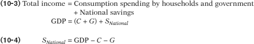
Since (GDP − C − G) is the amount of total income left over after consumption spending, it must be equal to savings for the economy as a whole. Making use of Equation (10-2), we get:
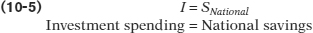
This is why we can say that it’s a basic accounting fact that savings equals investment spending for the economy as a whole.
Now, let’s take a closer look at national savings. As mentioned earlier, national savings comes from both households and the government. Thus, another way to look at national savings is to look at savings undertaken by each of these two sectors. Recall from Chapter 7 that the savings undertaken by households is called private savings, SPrivate, and this amount is equal to disposable income minus (private sector) consumption spending:

where GDP represents income, T represents taxes, and TR represents transfers from the government.
Public savings (or government budget balance) is the difference between net tax revenue (T − TR) and government spending on goods and services, i.e., T − TR − G. If the budget balance is positive, then the government is running a budget surplus. If it is negative, then the government is running a budget deficit. If it is zero, then the government is running a balanced budget.
As alluded to above, the government can also save. The savings by the government is usually called public savings, SPublic, but you may also see it referred to as government savings. Public savings is the government’s budget balance—that is, does the budget have a surplus or a deficit, or does total income equal total spending. Like households, the government earns income and has spending on goods and services. The government’s income consists of the tax revenues it collects, while its expenditures include spending on final goods and services and making transfer payments to residents. Sometimes, it is convenient to refer to the difference between the tax revenues and transfer payments as net taxes, in essence treating transfer payments as negative taxes. Thus, the government’s budget balance is the difference between the net tax revenue and government spending on final goods and services. If net taxes exceed government spending on final goods and services, then the government is running a budget surplus. Since the budget balance is positive, the government has saved the leftover. On the other hand, if the budget balance is negative, the government runs a budget deficit, or “dissaves,” as the government is engaged in the opposite of savings. Therefore, the budget balance of the government is equivalent to public savings:

National savings can be expressed as the sum of private savings and public savings:

Substituting Equations (10-6) and (10-7) into Equation (10-8), we get back Equation (10-4):
The Savings-
Net foreign investment (NFI) is the total outflows of funds out of a country minus the total inflows of funds into that country. It can also be expressed as the difference between the amount of foreign investment undertaken by the country and the amount of domestic investment undertaken by foreigners.
The net effect of international outflows and inflows of funds on total savings available for investment in any given country is known as the net foreign investment (NFI) of that country. NFI is equal to the total outflows of domestic funds minus the total inflows of foreign funds.1 Like the government budget balance, net foreign investment can be negative—
It’s important to note that, from a national perspective, a dollar generated by national savings and a dollar generated by a foreign capital inflow are not equivalent. Yes, they can both finance the same dollar’s worth of investment spending. But any dollar borrowed from a saver must eventually be repaid with interest. A dollar that comes from national savings is repaid with interest to someone domestically—
The fact that a negative net foreign investment represents funds “borrowed” from foreigners is an important aspect of the savings-

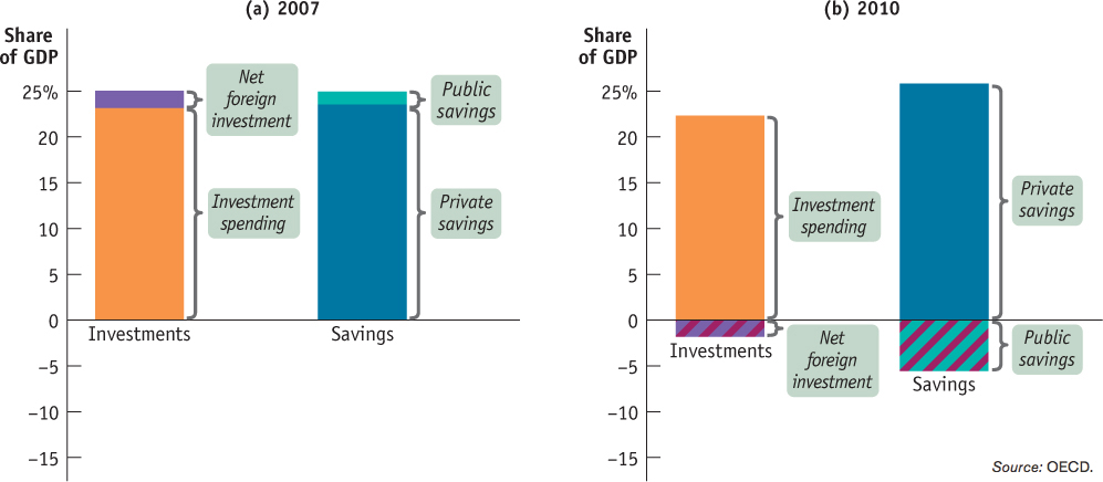
Rearranging Equation 10-1 we get:

The left side of Equation 10-10 is equal to national savings (Equation 10-4), so then:

Equation 10-11 shows that an open economy can split its savings into domestic investment (I) and net foreign investment (NFI). Let’s look at some data to demonstrate this. In 2010 in Canada, private savings reached $420.7 billion, while public savings were negative $90.2 billion. So, the government ran a budget deficit. This resulted in national savings of $330.5 billion. However, investment spending totalled $360.7 billion, which was greater than the amount of domestic funds available. The shortfall in funds was supplemented by a trade deficit of $30.5 billion. Thus, in 2010 Canada “borrowed” $30.5 billion from foreigners. You may have noticed these numbers don’t quite add up; because data collection isn’t perfect, there is a statistical discrepancy of $0.3 billion. But we know that the error lies in the data, not in the theory, because the savings-
THE DIFFERENT KINDS OF CAPITAL
It’s important to understand clearly the three different kinds of capital: physical capital, human capital, and financial capital (as explained in the previous chapter):
Physical capital consists of manufactured resources such as buildings and machines.
Human capital is the improvement in the labour force generated by education and knowledge.
Financial capital is funds from savings that are available for investment spending. A country that has a negative net foreign investment is experiencing a positive net flow of funds into that country from abroad, that is, from foreigners. These funds can be used to finance domestic investment spending.
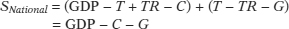
Figure 10-1 shows the savings-
Source: OECD.
Public savings changed from a positive 1.4% in 2007 to a negative 5.6% in 2010, which indicated the government’s budget balance changed from a surplus to a deficit. This change in budget balance was the result of an economic slowdown coupled with expansionary fiscal policies such as the Economic Action Plan and other programs implemented in response to the financial crisis. The increase in government spending, the provision of higher transfer payments, and a fall in tax revenues combined to force the federal government to run record-
Similarly, Canada’s net foreign investment changed from a positive 1.9% in 2007 to a negative 1.9% in 2010. In 2007, Canada experienced positive NFI and “lent” money to foreigners; in 2010, Canada experienced negative NFI and “borrowed” from foreigners. The change in the nature of NFI also indicated that Canada’s trade balance changed from a surplus to a deficit. This change was caused partly by the recession in the United States, which lowered the demand for exported Canadian goods, and partly by falling oil prices.
WHO ENFORCES THE ACCOUNTING?
The savings-
The short answer is that actual and desired investment spending aren’t always equal. Suppose that households suddenly decide to save more by spending less—
Let’s take a look at what happened in 2010. National savings and investment (the sum of domestic and net foreign investment) both increased by $24 billion from the fourth quarter of 2009 to the second quarter of 2010. On the investment side, $12 billion of that rise took the form of inventory investment spending, showing that when households save more and spend less, the resulting increase in unsold products leads to an increase in firms’ inventories. (So, for example, unsold automobiles continued to sit on the dealers’ lots.)
Of course, businesses respond to changes in their inventories by altering their production. The increase in inventories in 2010 helped to explain the slower GDP growth in the subsequent quarters, as firms responded by laying off workers and reducing output. We’ll examine the special role of inventories in economic fluctuations in Chapter 11.
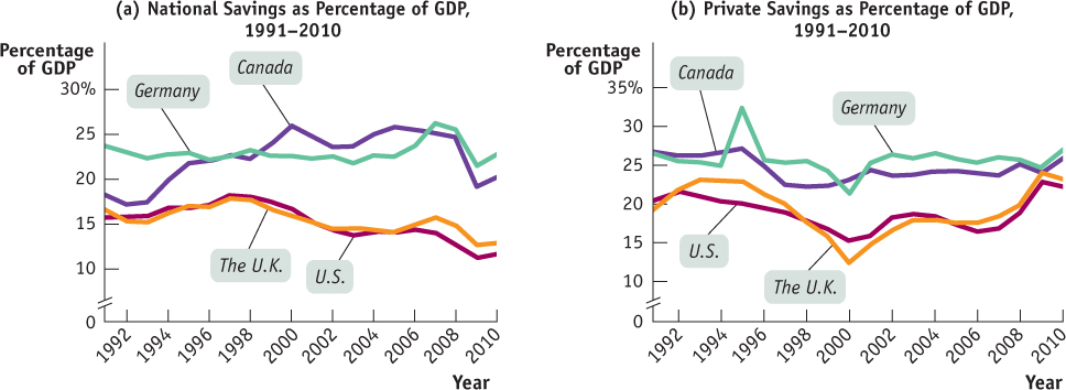
DIFFERENCES IN NATIONAL SAVINGS
Panel (a) of this figure shows national savings as a percentage of GDP for Canada, the United States, Germany, and the United Kingdom from 1991 to 2010. Canada’s and Germany’s savings rates were always higher than those of the U.S. and the U.K. The average national savings rates over that period were 22.5% (of GDP) in Canada and 23% in Germany; however, the average national savings rates in the U.S. and the U.K. were 15.2% and 15.4% respectively.
What causes the differences in savings rates among these countries? The main source of these international differences in national savings lies in the relatively low private savings in both the U.S. and the U.K. As panel (b) shows, before the recession of 2008–2009, American and British citizens saved much less than Canadians and Germans. Why? Economists aren’t sure, but one explanation is that U.S. and U.K. households have easier access to credit than Canadian and German households do. When households see that it is relatively easy to borrow to finance the purchase of big-
All four countries saw a drop in national savings rates after 2008. As one might expect, this drop was triggered by the financial crisis of 2008–2009; governments in all these countries ran expansionary fiscal policies (and budget deficits) to prevent their economies from taking a drastic downturn. As a result, the recent rise in private savings was more than offset by the fall in public savings.
Source: OECD.
On the other hand, the private sector saved more as a percentage of GDP over that period. Private savings increased from 23.7% of GDP in 2007 to 25.9% in 2010. This may have been triggered by heightened uncertainty about the future. Perhaps seeing that economic growth had slowed and firms were laying off workers as a result of the recent recession, households saved more for future rainy days! Although private savings as a percentage of GDP was higher in 2010, national savings actually fell to 20.3% of GDP as the increase in private savings was more than offset by a fall in public savings.
The Domestic Market for Loanable Funds
For the economy as a whole, savings always equals investment spending. In a closed economy, savings is equal to national savings. In an open economy, savings can be split between investment and net foreign investment. At any given time, however, savers, the people with funds to lend, are usually not the same as borrowers, the people who want to borrow to finance their investment spending. How are savers and borrowers brought together?
Savers and borrowers are matched up with one another in much the same way producers and consumers are matched up: through markets governed by supply and demand. In Figure 7-1, the expanded circular-flow diagram, we noted that the financial markets channel the savings of households to businesses that want to borrow in order to purchase capital equipment. It’s now time to take a look at how those financial markets work.
To do this, it helps to consider a somewhat simplified version of reality. As we noted in Chapter 7, there are a large number of different financial markets in the financial system, such as the bond market and the stock market. However, economists often work with a simplified model in which they assume that there is just one market that brings together those who want to lend money (savers) and those who want to borrow (firms with investment spending projects). This hypothetical market is known as the loanable funds market. The price that is determined in the loanable funds market is the interest rate, denoted by i. As we noted in Chapter 8, loans typically specify a nominal interest rate. So although we call i “the interest rate,” it is with the understanding that i is a nominal interest rate—an interest rate that is unadjusted for inflation.
The loanable funds market is a hypothetical market that illustrates the market outcome of the demand for funds generated by borrowers and the supply of funds provided by lenders.
We’re not quite done simplifying things. There are, in reality, many different kinds of interest rates, because there are many different kinds of loans—short-term loans, long-term loans, loans made to corporate borrowers, loans made to governments, and so on. In the interest of simplicity, we’ll ignore those differences and assume that there is only one type of loan.
OK, now we’re ready to analyze how savings and investment get matched up.
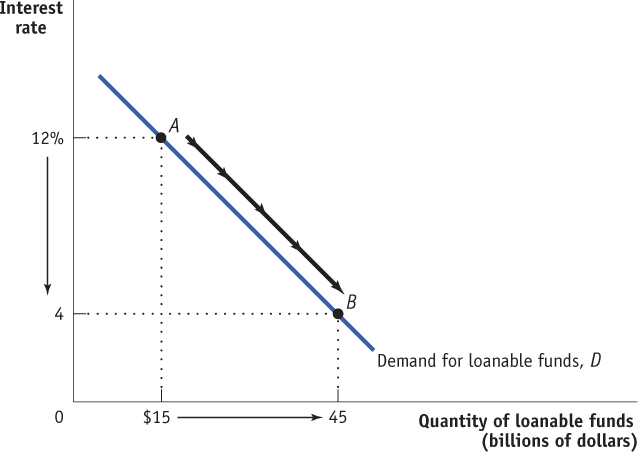
The Domestic Demand for Loanable Funds The domestic demand for loanable funds (or, for short, the demand for loanable funds) comes from those who need to borrow funds to finance their domestic investment project(s). Figure 10-2 illustrates a hypothetical demand curve for loanable funds, D, which slopes downward. On the horizontal axis we show the quantity of loanable funds demanded. On the vertical axis we show the interest rate, which is the “price” of borrowing. But why does the demand curve for loanable funds slope downward?
USING PRESENT VALUE
An understanding of the concept of present value shows why the demand curve for loanable funds slopes downward. A simple way to grasp the essence of present value is to consider an example that illustrates the difference in value between having a sum of money today and having the same sum of money a year from now.
Suppose that exactly one year from today you will graduate, and you want to reward yourself by taking a trip that will cost $1000. In order to have $1000 a year from now, how much do you need today? It’s not $1000, and the reason why has to do with the interest rate. Let’s call the amount you need today X. We’ll use i to represent the interest rate you receive on funds deposited in the bank. If you put X into the bank today and earn interest rate i on it, then after one year, the bank will pay you X × (1 + i). If what the bank will pay you a year from now is equal to $1000, then the amount you need today is

You can apply some basic algebra to find that

Notice that the value of X depends on the interest rate i, which is always greater than 0. This fact implies that X is always less than $1000. For example, if i = 5% (that is, i = 0.05), then X = $952.38. In other words, having $952.38 today is equivalent to having $1000 a year from now when the interest rate is 5%. That is, $952.38 is the present value of having $1000 a year from now when the interest rate is 5%. Now we can define the present value of X: it is the amount of money needed today in order to receive X in the future given the interest rate. In this numerical example, $952.38 is the present value of $1000 received one year from now given an interest rate of 5%.
The present value of Y dollars is the amount of money you would need to invest today at the given interest rate to receive Y dollars at a future date.

The concept of present value also applies to decisions made by firms. Think about a firm that has two potential investment projects in mind, each of which will yield $1000 a year from now. However, each project has different initial costs—say, one requires that the firm borrow $900 right now and the other requires that the firm borrow $950. Which, if any, of these projects is worth borrowing money to finance and undertake?
The answer depends on the interest rate, which determines the present value of $1000 a year from now. If the interest rate is 10%, the present value of $1000 delivered a year from now is $909. So only the first project, which has an initial cost of less than $909, is profitable. With an interest rate of 10%, the return on any project costing more than $909 is less than the amount the firm had to repay on its loan and is therefore unprofitable. If the interest rate is only 5%, however, the present value of $1000 rises to $952. At this interest rate, both projects are profitable because $952 exceeds both projects’ initial cost. So a firm will want to borrow more (i.e., demand more funds) and engage in more investment spending when the interest rate is lower.
Meanwhile, similar calculations will be taking place at other firms. So a lower interest rate will lead to higher investment spending in the economy as a whole: the demand curve for loanable funds slopes downward.
To answer this question, consider what a firm is doing when it engages in investment spending—say, by buying new equipment. Investment spending means laying out money right now, expecting that this outlay will lead to higher profits at some point in the future. In fact, however, the promise of a dollar five or ten years from now is worth less than an actual dollar right now. So an investment is worth making only if it generates a future return that is greater than the monetary cost of making the investment today. How much greater? To answer that, we need to take into account the present value of the future return the firm expects to get. We examine the concept of present value in the accompanying For Inquiring Minds.
In present value calculations, we use the interest rate to determine how the value of a dollar in the future compares to the value of a dollar today. But the fact is that future dollars are worth less than a dollar today, and they are worth even less when the interest rate is higher. The intuition behind present value calculations is simple. The interest rate measures the opportunity cost of investment spending that results in a future return: instead of spending money on an investment spending project, a company could simply put the money into the bank and earn interest on it. And the higher the interest rate, the more attractive it is to simply put money into the bank instead of investing it in an investment spending project. In other words, the higher the interest rate, the higher the opportunity cost of investment spending. And, the higher the opportunity cost of investment spending, the lower the number of investment spending projects firms want to carry out, and therefore the lower the quantity of loanable funds demanded. It is this insight (discussed in the accompanying For Inquiring Minds) that explains why the demand curve for loanable funds is downward sloping.
When businesses engage in investment spending, they spend money right now in return for an expected payoff in the future. So, to evaluate whether a particular investment spending project is worth undertaking, a business must compare the present value of the future payoff with the current cost of that project. If the present value of the future payoff is greater than the current cost, a project is profitable and worth investing in. If the interest rate falls, then the present value of any given project rises, so more projects pass that test. If the interest rate rises, then the present value of any given project falls, then fewer projects pass that test. So total investment spending, and hence the demand for loanable funds to finance that spending, is negatively related to the interest rate. Thus, the demand curve for loanable funds slopes downward. You can see this in Figure 10-2. When the interest rate falls from 12% to 4%, the quantity of loanable funds demanded rises from $15 billion (point A) to $45 billion (point B).
The Domestic Supply of Loanable Funds The domestic supply of loanable funds (or, for short, the supply of loanable funds) comes from those who have extra funds that they are willing to lend. This supply is equal to national savings. Figure 10-3 shows a hypothetical supply curve for loanable funds, S. Again, the interest rate plays the same role that the price plays in ordinary supply and demand analysis. But why is this curve upward sloping?
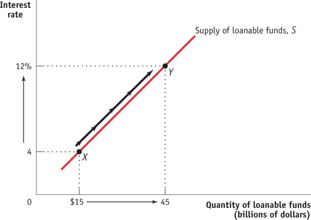
The answer is that loanable funds are supplied by savers, and savers incur an opportunity cost when they lend to a business: the funds could instead be spent on consumption—say, a nice vacation. Whether a given saver becomes a lender by making funds available to borrowers depends on the interest rate received in return. By saving your money today and earning interest on it, you are rewarded with higher consumption in the future when the loan you made is repaid with interest. So it is a good assumption that more people are willing to forgo current consumption and make a loan to a borrower when the interest rate is higher. As a result, our hypothetical supply curve of loanable funds slopes upward. In Figure 10-3, lenders will supply $15 billion to the loanable funds market at an interest rate of 4% (point X); if the interest rate rises to 12%, the quantity of loanable funds supplied will rise to $45 billion (point Y).
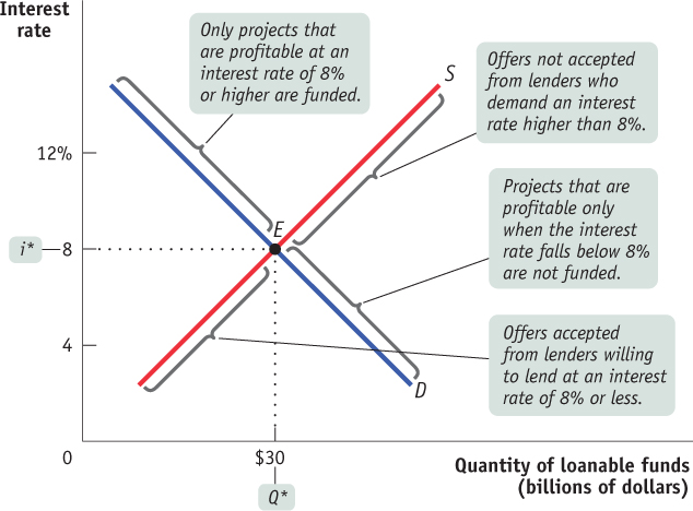
The Equilibrium Interest Rate The equilibrium interest rate is the interest rate at which the quantity of loanable funds supplied equals the quantity of loanable funds demanded. As you can see in Figure 10-4, the equilibrium interest rate, i*, and the total quantity of lending, Q*, are determined by the intersection of the supply and demand curves, at point E. Here, the equilibrium interest rate is 8%, at which $30 billion is lent and borrowed. In this equilibrium, only investment spending projects that are profitable if the interest rate is 8% or higher are funded. Projects that are profitable only when the interest rate falls below 8% will not be funded. Correspondingly, only lenders who are willing to accept an interest rate of 8% or less will have their offers to lend funds accepted; lenders who demand an interest rate higher than 8% do not have their offers to lend accepted.
Figure 10-4 shows how the market for loanable funds matches up desired savings with desired investment spending: in equilibrium, the quantity of funds that savers want to lend is equal to the quantity of funds that firms want to borrow (point E). The figure also shows that this match-up is efficient, in two senses. First, the right investments get made: the investment spending projects that are actually financed have higher payoffs (in terms of present value) than those that do not get financed. Second, the right people do the saving and lending: the savers who actually lend funds are willing to lend for lower interest rates than those who do not.
The insight that the loanable funds market leads to an efficient use of savings, although drawn from a highly simplified model, has important implications for real life. As we’ll see shortly, it is the reason that a well-functioning financial system increases an economy’s long-run economic growth rate.
Before we get to that, let’s look at how the market for loanable funds responds to shifts of demand and supply. As in the standard model of supply and demand, where the equilibrium price changes in response to shifts of the demand or supply curves, here the equilibrium interest rate changes when there are shifts of the demand curve for loanable funds, the supply curve for loanable funds, or both.
Shifts of the Domestic Demand for Loanable Funds Let’s start by looking at the causes and effects of changes in demand.
The factors that can cause the demand curve for loanable funds to shift include the following:
Changes in perceived business opportunities. A change in beliefs about the payoff of investment spending can increase or reduce the amount of desired investment spending at any given interest rate. For example, during the 1990s there was great excitement over the business possibilities created by the Internet, which had just begun to be widely used. As a result, businesses rushed to buy computer equipment, put fibre optic cables in the ground, and so on. This shifted the demand for loanable funds to the right. By 2001, the failure of many dot-com businesses had led to disillusionment with technology-related investment; this shifted the demand for loanable funds back to the left.
Changes in government policies that affect investment. Government policies toward investment can affect business and household incentives to undertake investment. One such policy is a tax credit for investment. A tax credit is a subsidy in the form of lower taxes for those undertaking the targeted type of investment. This policy would promote investment as investment becomes more attractive (less expensive to undertake) for decision-makers. As a result, more investment projects will be undertaken at any given level of the interest rate. So, holding all else constant, the provision of an investment tax credit shifts the demand for loanable funds to the right.
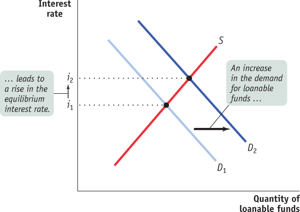
Figure 10-5 shows the effects of an increase in the demand for loanable funds. S is the supply of loanable funds, and D1 is the initial demand curve. The initial equilibrium interest rate is i1. An increase in the demand for loanable funds means that the quantity of funds demanded rises at any given interest rate, so the demand curve shifts rightward to D2. As a result, the equilibrium interest rate rises to i2.
Shifts of the Domestic Supply of Loanable Funds Like the demand for loanable funds, the supply of loanable funds can shift. Among the factors that can cause the supply of loanable funds to shift are the following:
Changes in private savings behaviour. A number of factors can cause the level of private savings to change at any given interest rate. For example, rising home prices in Canada in the past decade made many homeowners feel richer, making them willing to spend more and save less. This had the effect of shifting the supply curve of loanable funds to the left.
Changes in government budget balance. Recall that national savings come from two sources: the private sector and governments. When the government runs a budget surplus, public savings are positive. These savings from the government can be used to finance investment spending. Similarly, when the government runs a budget deficit, public savings are negative and there will be a reduction in national savings. Thus, changes in the government budget balance can shift the supply of loanable funds. For example, the federal budgetary balance went from a surplus of $15.4 billion in 2007 to a deficit of $33 billion in 2009. This change in budget balance means that the federal government went from being a net saver that provided loanable funds to the market to being a net borrower. Holding all else constant, this change in budget balance will lower national savings and reduce the amount of loanable funds available. As a result, the supply of loanable funds shifts to the left.
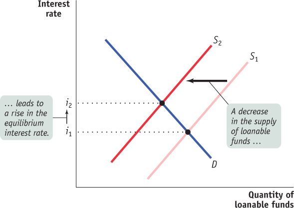
Figure 10-6 shows the effects of a decrease in the supply of loanable funds. D is the demand for loanable funds, and S1 is the initial supply curve. The initial equilibrium interest rate is i1. A decrease in the supply of loanable funds means that the quantity of funds supplied falls at any given interest rate, so the supply curve shifts leftward to S2. As a result, the equilibrium interest rate rises to i2.
The fact that a reduction in the supply of loanable funds leads, other things equal, to a rise in the interest rate has one especially important implication: it tells us that increasing or persistent government budget deficits are cause for concern because an increase in the government’s deficit shifts the supply curve of loanable funds to the left, which leads to a higher interest rate. If the interest rate rises, businesses and households will cut back on their investment spending. So, other things equal, a rise in the government budget deficit tends to reduce overall investment spending. Economists call the negative effect of government budget deficits on investment spending crowding out. It is a key reason for worry about increasing or persistent budget deficits, which explains why a government might put balancing the budget as one of its top priorities.2
Crowding out occurs when a government budget deficit drives up the interest rate and leads to reduced investment spending.
Inflation and Interest Rates Anything that shifts either the supply of loanable funds curve or the demand for loanable funds curve changes the interest rate. Historically, major changes in interest rates have been driven by many factors, including changes in government policy and technological innovations that created new investment opportunities. However, arguably the most important factor affecting interest rates over time—the reason, for example, that interest rates today are much lower than they were in the late 1970s and early 1980s—is changing expectations about future inflation, which shift both the supply and the demand for loanable funds.
To understand the effect of expected future inflation on interest rates, recall our discussion in Chapter 8 of the way inflation creates winners and losers—for example, the way that higher than expected Canadian inflation in the 1970s and 1980s reduced the real value of homeowners’ mortgages, which was good for the homeowners but bad for the banks. In Chapter 8 we learned that economists summarize the effect of inflation on borrowers and lenders by distinguishing between the nominal interest rate and the real interest rate, where the difference is:

The true cost of borrowing is the real interest rate, not the nominal interest rate. To see why, suppose a firm borrows $10 000 for one year at a 10% nominal interest rate. At the end of the year, it must repay $11 000—the amount borrowed plus the interest. But suppose that over the course of the year the average level of prices increases by 10%, so that the real interest rate is zero. Then the $11 000 repayment has the same purchasing power as the original $10 000 loan. In real terms, the borrower has received a zero-interest loan.
Similarly, the true payoff to lending is the real interest rate, not the nominal rate. Suppose that a bank makes a $10 000 loan for one year at a 10% nominal interest rate. At the end of the year, the bank receives an $11 000 repayment. But if the average level of prices rises by 10% per year, the purchasing power of the money the bank gets back is no more than that of the money it lent out. In real terms, the bank has made a zero-interest loan.
Now we can add an important detail to our analysis of the loanable funds market. Figures 10-5 and 10-6 are drawn with the vertical axis measuring the nominal interest rate for a given expected future inflation rate. Why do we use the nominal interest rate rather than the real interest rate? Because in the real world neither borrowers nor lenders know what the future inflation rate will be when they make a deal. Actual loan contracts therefore specify a nominal interest rate rather than a real interest rate. Because we are holding the expected future inflation rate fixed in Figures 10-5 and 10-6, however, changes in the nominal interest rate also lead to changes in the real interest rate.
The expectations of borrowers and lenders about future inflation rates are normally based on recent experience. In the late 1970s, after a decade of high inflation, borrowers and lenders expected future inflation to be high. By the late 1990s, after a decade of fairly low inflation, borrowers and lenders expected future inflation to be low. And these changing expectations about future inflation had a strong effect on the nominal interest rate, largely explaining why nominal interest rates were much lower in the early years of the twenty-first century than they were in the early 1980s.
Let’s look at how changes in the expected future rate of inflation are reflected in the loanable funds model.
In Figure 10-7, the curves S0 and D0 show the supply and demand for loanable funds given that the expected future rate of inflation is 0%. In that case, equilibrium is at E0 and the equilibrium nominal interest rate is 4%. Because expected future inflation is 0%, the equilibrium expected real interest rate over the life of the loan is also 4%.
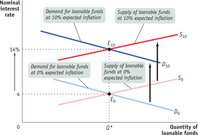
Now suppose that the expected future inflation rate rises to 10%. The demand curve for loanable funds shifts upward to D10: borrowers are now willing to borrow as much at a nominal interest rate of 14% as they were previously willing to borrow at 4%. That’s because with a 10% inflation rate, a 14% nominal interest rate corresponds to a 4% real interest rate. Similarly, the supply curve of loanable funds shifts upward to S10: lenders require a nominal interest rate of 14% to persuade them to lend as much as they would previously have lent at 4%. The new equilibrium is at E10: the result of an expected future inflation rate of 10% is that the equilibrium nominal interest rate rises from 4% to 14%.
This situation can be summarized as a general principle, known as the Fisher effect (after the American economist Irving Fisher, who proposed it in 1930): In the long run, the expected real interest rate is unaffected by changes in expected future inflation. According to the Fisher effect, an increase in expected future inflation drives up the nominal interest rate, where each additional percentage point of expected future inflation drives up the nominal interest rate by 1 percentage point. The central point is that both lenders and borrowers base their decisions on the expected real interest rate. As a result, a change in the expected rate of inflation does not affect the equilibrium quantity of loanable funds or the expected real interest rate; all it affects is the equilibrium nominal interest rate.
According to the Fisher effect, an increase in expected future inflation drives up the nominal interest rate, leaving the expected real interest rate unchanged.
FIFTY YEARS OF CANADIAN INTEREST RATES
There have been some large movements in Canada’s interest rates over the past half-century. These movements clearly show how changes both in expected future inflation and in the expected return on investment spending move interest rates in the longer term.
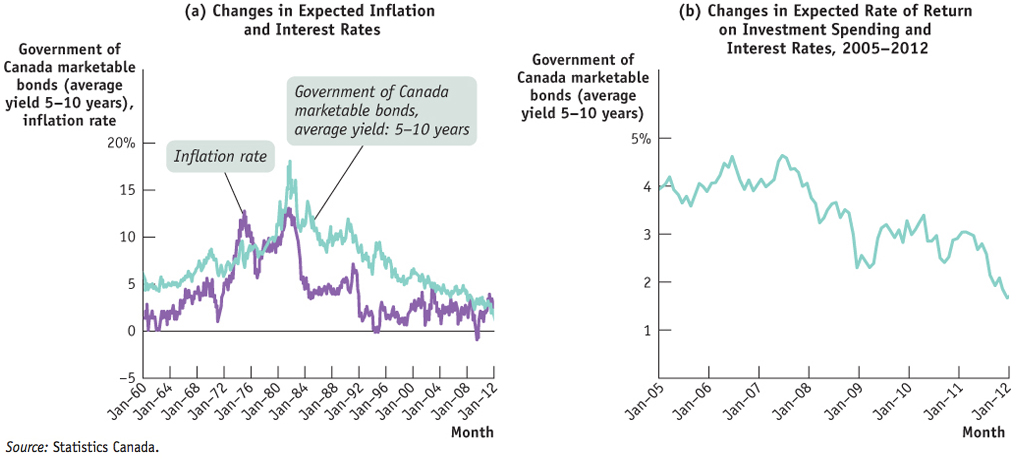
Figure 10-8a illustrates the first effect. It shows the average interest rate on bonds issued by the Government of Canada—specifically, bonds for which the government promises to repay the full amount in the longer term (5–10 years later)—from 1960 to 2012, along with the rate of consumer price inflation over the same period. As you can see, the big story about interest rates is the way they soared in the 1970s, before coming back down in the 1980s. It’s not hard to see why that happened: inflation shot up during the 1970s, leading to widespread expectations that high inflation would continue. And as we’ve seen, expected inflation raises the equilibrium (nominal) interest rate. As inflation came down in the 1980s, so did expectations of future inflation, and this brought interest rates down as well.
Source: Statistics Canada.
Figure 10-8b illustrates the second effect: changes in the expected return on investment spending and interest rates, with a “close-up” of interest rates from 2005 to 2012. Notice the sharp drop in interest rate in mid-2007. We know from other evidence that expected inflation didn’t change much over those years as the Bank of Canada has an explicitly stated inflation target of 2%. What happened, instead, was a change in the attitudes of businesses (and households) toward investment. In 2007, it was becoming increasingly evident that the housing bubble in the U.S. was about to burst. The economies of Canada and America are closely related, so of course a slowdown in the American economy would cause our economy to slow down as well. As a result, Canadian businesses became more cautious about investing. They reasoned that if an economic slowdown did occur, the return on investment would be less attractive. When businesses became more pessimistic about the future economic outlook, there was a leftward shift in the demand for loanable funds and a fall in the interest rate.
Throughout this whole process, total savings was equal to total investment spending, and the rise and fall of the interest rate played a key role in matching lenders with borrowers.

Quick Review
The savings-investment spending identity is an accounting fact: savings is equal to investment spending for the economy as a whole.
The government is a source of savings when it runs a positive budget balance, a budget surplus. Public savings is the government’s budget balance. The government is a source of dissavings when it runs a negative budget balance, a budget deficit.
National savings must equal investment spending in a closed economy. However, in an open economy, national savings can be split between investment spending and net foreign investment, which may be positive, zero, or negative.
When costs or benefits arrive at different times, you must take the complication created by time into account. This is done by transforming any dollars realized in the future into their present value.
The loanable funds market matches savers to borrowers. In equilibrium, only investment spending projects with an expected return greater than or equal to the equilibrium interest rate are funded.
A government budget deficit will lower the country’s national savings—shifting the supply of loanable funds in the market to the left. This drives up the interest rate and reduces investment in equilibrium. Therefore, a government deficit can cause crowding out.
Higher expected future inflation raises the nominal interest rate through the Fisher effect, leaving the real interest rate unchanged in the long run.
Check Your Understanding 10-1
CHECK YOUR UNDERSTANDING 10-1
Question 10.1
Use a diagram of the loanable funds market to illustrate the effect of the following events on the equilibrium interest rate and investment spending.
The government reduces a subsidy to investment.
Retired people generally save less than working people at any interest rate. The proportion of retired people in the population goes up.
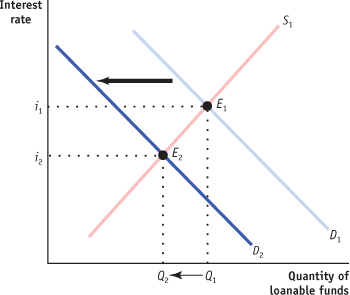
When the government reduces its subsidy on investment, this makes undertaking investment becomes less attractive, and the demand for loanable funds decreases. This is illustrated by the shift of the demand curve from D1 to D2 in the accompanying diagram. As the equilibrium moves from E1 to E2, the equilibrium interest rate falls from i1 to i2, and the equilibrium quantity of loanable funds decreases from Q1 to Q2.
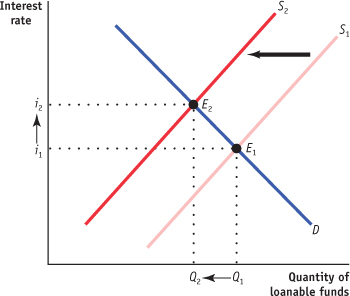
Savings fall due to the higher proportion of retired people, and the supply of loanable funds decreases. This is illustrated by the leftward shift of the supply curve from S1 to S2 in the accompanying diagram. The equilibrium moves from E1 to E2, the equilibrium interest rate rises from i1 to i2, and the equilibrium quantity of loanable funds falls from Q1 to Q2.
Question 10.2
Explain what is wrong with the following statement: “Savings and investment spending may not be equal in the economy as a whole because when the interest rate rises, households will want to save more money than businesses will want to invest.”
We know from the loanable funds market that as the interest rate rises, households want to save more and consume less. But at the same time, an increase in the interest rate lowers the number of investment spending projects with returns at least as high as the interest rate. The statement “households will want to save more money than businesses will want to invest” cannot represent an equilibrium in the loanable funds market because it says that the quantity of loanable funds offered exceeds the quantity of loanable funds demanded. If that were to occur, the interest rate must fall to make the quantity of loanable funds offered equal to the quantity of loanable funds demanded.
Question 10.3
Suppose that expected inflation rises from 3% to 6%.
How will the real interest rate be affected by this change?
How will the nominal interest rate be affected by this change?
What will happen to the equilibrium quantity of loanable funds?
The real interest rate will not change. According to the Fisher effect, an increase in expected inflation drives up the nominal interest rate, leaving the real interest rate unchanged.
The nominal interest rate will rise by 3%. Each additional percentage point of expected inflation drives up the nominal interest rate by 1 percentage point.
As we saw in Figure 10-7, as long as inflation is expected, it does not affect the equilibrium quantity of loanable funds. Both the supply and demand curves for loanable funds are pushed upward, leaving the equilibrium quantity of loanable funds unchanged.