11.1 The Multiplier: An Informal Introduction
The story of the boom and bust in the cod fishery involves a sort of chain reaction in which an initial rise or fall in aggregate expenditure leads to changes in income, which lead to further changes in aggregate expenditure, and so on. Let’s examine that chain reaction more closely, this time thinking through the effects of changes in aggregate expenditure on the economy as a whole.
For the sake of this analysis, we’ll make four simplifying assumptions that will have to be reconsidered in later chapters.
We assume that producers are willing to supply additional output at a fixed price. That is, if consumers or businesses buying investment goods decide to spend an additional $1 billion, that will translate into the production of $1 billion worth of additional goods and services without driving up the overall level of prices. As a result, changes in aggregate expenditure translate into changes in aggregate output, as measured by real GDP. As we’ll learn in the next chapter, this assumption isn’t too unrealistic in the short run, but it needs to be changed when we think about the long-
run effects of changes in demand. We take the interest rate as given.
We assume that there is no government spending, no taxes, and no transfer payments.
We assume that exports and imports are zero.
Given these simplifying assumptions, consider what happens if there is a change in investment spending. Specifically, imagine that for some reason home builders decide to spend an extra $10 billion on home construction over the next year.
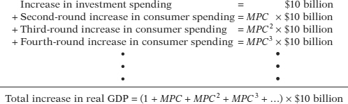
The direct effect of this increase in investment spending will be to increase income and the value of aggregate output by the same amount. That’s because each dollar spent on home construction translates into a dollar’s worth of income for construction workers, suppliers of building materials, electricians, and so on. If the process stopped there, the increase in housing investment spending would raise overall income by exactly $10 billion.
But the process doesn’t stop there. The increase in aggregate output leads to an increase in disposable income that flows to households in the form of profits and wages. The increase in households’ disposable incomes leads to a rise in consumer spending, which, in turn, induces firms to increase output yet again. This generates another rise in disposable income, which leads to another round of consumer spending increases, and so on. So there are multiple rounds of increases in aggregate output.
How large is the total effect on aggregate output if we sum the effect from all these rounds of spending increases? To answer this question, we need to introduce the concept of the marginal propensity to consume, or MPC: the increase in consumer spending when disposable income rises by $1. When consumer spending changes because of a rise or fall in disposable income, MPC is the change in consumer spending divided by the change in disposable income:
The marginal propensity to consume, or MPC, is the increase in consumer spending when disposable income rises by $1. MPC is a positive fraction less than 1, i.e., 0 < MPC < 1.

where the symbol Δ (delta) means “change in.” For example, if consumer spending goes up by $6 billion when disposable income goes up by $10 billion, MPC is $6 billion/$10 billion = 0.6.
The marginal propensity to save, or MPS, is the increase in household savings when disposable income rises by $1. MPS is also a positive fraction less than 1, i.e., 0 < MPS < 1, and MPC + MPS = 1.
Because consumers normally spend part but not all of an additional dollar of disposable income, MPC is a number between 0 and 1. The additional disposable income that consumers don’t spend is saved; the marginal propensity to save, or MPS, is the fraction of an additional dollar of disposable income that is saved. MPS is equal to 1 − MPC.
Because we assumed that there are no taxes and no international trade, each $1 increase in aggregate expenditure raises both real GDP and disposable income by $1. So the $10 billion increase in investment spending initially raises real GDP by $10 billion. This leads to a second-
So the $10 billion increase in investment spending sets off a chain reaction in the economy. The net result of this chain reaction is that a $10 billion increase in investment spending leads to a change in real GDP that is a multiple of the size of that initial change in spending.
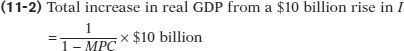
How large is this multiple? It’s a mathematical fact that an infinite series of the form 1 + x + x2 + x3 + …, where x is between 0 and 1, is equal to 1/(1 −x). So the total effect of a $10 billion increase in investment spending, I, taking into account all the subsequent increases in consumer spending (and assuming no taxes and no international trade), is given by:
Let’s consider a numerical example in which MPC = 0.6: each $1 in additional disposable income causes a $0.60 rise in consumer spending. In that case, a $10 billion increase in investment spending raises real GDP by $10 billion in the first round. The second-

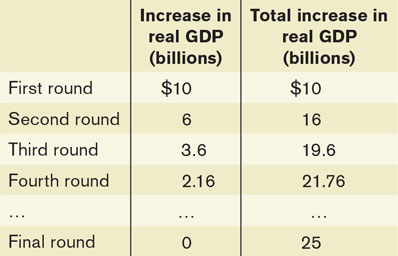
Notice that even though there are an infinite number of rounds of expansion of real GDP, the total rise in real GDP is limited to $25 billion. The reason is that at each stage some of the rise in disposable income “leaks out” because it is saved. How much of an additional dollar of disposable income is saved depends on MPS, the marginal propensity to save.
We’ve described the effects of a change in investment spending, but the same analysis can be applied to any other change in aggregate expenditure, such as consumer spending. The important thing is to distinguish between the initial change in aggregate expenditure, before real GDP rises, and the additional change in aggregate expenditure caused by the change in real GDP as the chain reaction unfolds. For example, suppose that a boom in housing prices makes consumers feel richer and that, as a result, they become willing to spend more at any given level of disposable income. This will lead to an initial rise in consumer spending, before real GDP rises. But it will also lead to second and later rounds of higher consumer spending as real GDP rises.
An autonomous change in aggregate expenditure is an initial change in the desired level of spending by firms, households, or government at a given level of real GDP.
An initial rise or fall in aggregate expenditure at a given level of real GDP is called an autonomous change in aggregate expenditure. It’s autonomous—
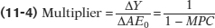
The multiplier is the ratio of the total change in real GDP caused by an autonomous change in aggregate expenditure to the size of that autonomous change.
So the multiplier is:
Notice that the size of the multiplier depends on MPC. If the marginal propensity to consume is high, so is the multiplier. This is true because the size of MPC determines how large each round of expansion is compared with the previous round. To put it another way, the higher MPC is, the less disposable income “leaks out” into savings at each round of expansion. Let’s return to our earlier example of a $100 billion increase in investment. If the MPC rises from 0.6 to 0.75, then the multiplier increases from 2.5 to 4, and the total possible increase in real GDP will be equal to $400 billion (an additional $150 billion increase in real GDP).
In later chapters we’ll use the concept of the multiplier to analyze the effects of fiscal and monetary policies. We’ll also see that the formula for the multiplier changes when we introduce various complications, including taxes and foreign trade. First, however, we need to look more deeply at what determines consumer spending.
THE MULTIPLIER AND THE GREAT DEPRESSION
The concept of the multiplier was originally devised by economists trying to understand the greatest economic disaster in history, the collapse of output and employment from 1929 to 1933, which began the Great Depression. Most economists believe that the slump during these years was caused by a collapse in investment spending. But as the economy shrank, consumer spending also fell sharply, multiplying the effect on real GDP.
Table 11-2 shows what happened to investment spending, consumer spending, and GDP during those five terrible years. All data are in 1971 dollars. Both consumer and investment spending fell during this period. Consumer spending fell by 18%, while investment spending plunged by more than 80%. The drastic fall in investment accounted for most of the reduction in real GDP. (The total fall in real GDP was smaller than the combined reduction in consumer and investment spending due to an improvement in the trade balance and technical accounting issues).
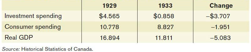
The numbers in Table 11-2 suggest that at the time of the Great Depression, Canada’s multiplier was around 1.4, whereas today it has risen significantly, to about 3. Why has there been such a change? In 1929, government in Canada was very small by modern standards: taxes were low and major government programs like employment insurance and health care had not yet come into being. In the modern Canadian economy, taxes are much higher, and so is government spending. Why does this matter? It matters since some taxes and government programs act as automatic stabilizers, reducing the size of the multiplier. Appendix 13A explains how taxes change the multiplier.

Quick Review
A change in investment spending arising from a change in expectations starts a chain reaction in which the initial change in real GDP leads to changes in consumer spending, leading to further changes in real GDP, and so on. The total change in aggregate output is a multiple of the initial change in investment spending.
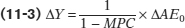
Any autonomous change in aggregate expenditure, a change in spending that is not caused by a change in real GDP, generates the same chain reaction. The total size of the change in real GDP depends on the size of the multiplier. Assuming that there are no taxes and no trade, the multiplier is equal to 1/(1 − MPC), where MPC is the marginal propensity to consume. The total change in real GDP, ΔY, is equal to 1/(1 − MPC) × ΔAE0.
Check Your Understanding 11-1
CHECK YOUR UNDERSTANDING 11-1
Question 11.1
Explain why a decline in investment spending caused by a change in business expectations leads to a fall in consumer spending.
A decline in investment spending, like a rise in investment spending, has a multiplier effect on real GDP—
Question 11.2
What is the multiplier if the marginal propensity to consume is 0.5? What is it if MPC is 0.8?
When the MPC is 0.5, the multiplier is equal to 1/(1 – 0.5) = 1/0.5 = 2. When the MPC is 0.8, the multiplier is equal to 1/(1 – 0.8) = 1/0.2 = 5.
Question 11.3
As a percentage of GDP, savings accounts for a larger share of the economy in the country of Scania compared to the country of Candia. Which country is likely to have the larger multiplier? Explain.
The greater the share of GDP that is saved rather than spent, the lower the MPC. Disposable income that goes to savings is like a “leak” in the system, reducing the amount of spending that fuels a further expansion. So it is likely that Amerigo will have the larger multiplier.