12.3 The AD-
From 1929 to 1933, the Canadian economy moved down the short-
In the AD-
So to understand the behaviour of the economy, we must put the aggregate supply curve and the aggregate demand curve together. The result is the AD-AS model, the basic model we use to understand economic fluctuations.
Short-Run Macroeconomic Equilibrium
We’ll begin our analysis by focusing on the short run. Figure 12-12 shows the aggregate demand curve and the short-
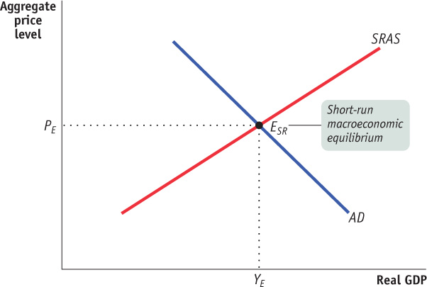
The economy is in short-run macroeconomic equilibrium when the quantity of aggregate output supplied in the short run is equal to the quantity demanded.
The short-run equilibrium aggregate price level is the aggregate price level in the short run macroeconomic equilibrium.
Short-run equilibrium aggregate output is the quantity of aggregate output produced in the short-
In the supply and demand model of Chapter 3 we saw that a shortage of any individual good causes its market price to rise but a surplus of the good causes its market price to fall. These forces ensure that the market reaches equilibrium. The same logic applies to short-
We’ll also make another important simplification based on the observation that in reality there is a long-
Short-
Shifts of Aggregate Demand: Short-Run Effects
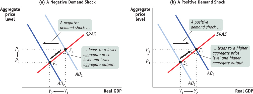
An event that shifts the aggregate demand curve is a demand shock.
An event that shifts the aggregate demand curve, such as a change in expectations or wealth, the effect of the size of the existing stock of physical capital, or the use of fiscal or monetary policy, is known as a demand shock. The Great Depression was caused by a negative demand shock, the collapse of wealth and of business and consumer confidence that followed the stock market crash of 1929 and the banking crisis of 1930-1931. The Depression was ended by a positive demand shock—
Figure 12-13 shows the short-
Shifts of the SRAS Curve
An event that shifts the short-
An event that shifts the short-
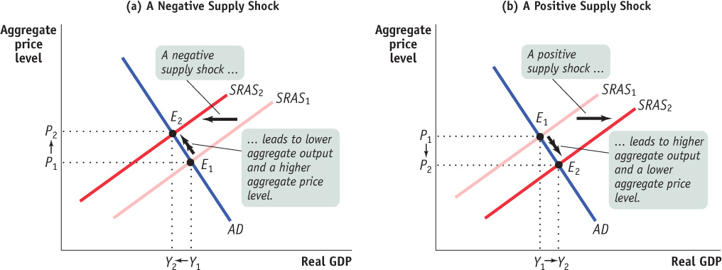
The effects of a negative supply shock to the short-
SUPPLY SHOCKS OF THE TWENTY-FIRST CENTURY
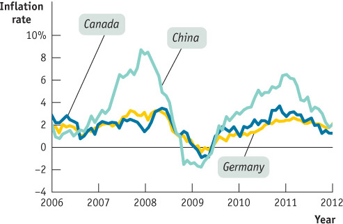
The price of oil and other raw materials has been highly unstable in recent years, with surging prices in 2007-2008, plunging prices in 2008-2009, and another surge starting in the second half of 2010. There is still controversy as to the reasons for these wild swings, but there is no disagreement about their macroeconomic impact: much of the world has been subjected to a series of supply shocks. There was a negative shock in 2007-2008, a positive shock in 2008-2009, and another negative shock in 20W-
You can see the effect of these shocks in the accompanying figure, which shows the rate of inflation, as measured by the percentage change in consumer prices over the previous year, in three economies. Economic policies have been quite different in Canada, Germany (which shares a currency with another ļ6 European countries), and China. Yet, in all three countries, inflation rose sharply in 2007-2008, fell dramatically thereafter, and rose sharply again in 2010–2011.
Stagflation is the combination of rising prices (higher inflation) and falling aggregate output.
The combination of rising prices (higher inflation) and falling aggregate output shown in panel (a) has a special name: stagflation, for “stagnation plus inflation.” When an economy experiences stagflation, it’s very unpleasant: falling aggregate output leads to rising unemployment, and people feel that their purchasing power is squeezed by rising prices. Stagflation in the 1970s led to a mood of national pessimism. It also, as we’ll see shortly, poses a dilemma for policy-

A positive supply shock, shown in panel (b), has exactly the opposite effects. A rightward shift of the SRAS curve from SRAS1 to SRAS2 results in a rise in aggregate output and a fall in the aggregate price level, a downward movement along the AD curve. The favourable supply shocks of the late 1990s led to a combination of higher employment and lower prices compared with the long-
The distinctive feature of supply shocks, both negative and positive, is that, unlike demand shocks, they cause the aggregate price level and aggregate output to move in opposite directions.
There’s another important contrast between supply shocks and demand shocks. As we’ve seen, monetary policy and fiscal policy enable the government to shift the AD curve, meaning that governments are in a position to create the kinds of shocks shown in Figure 12-13. It’s much harder for governments to shift the AS curve. Are there good policy reasons to shift the AD curve? We’ll turn to that question soon.
Simultaneous Shifts of the SRAS and LRAS Curves
As noted in Tables 12-2 and 12-3, changes in productivity can shift both the SRAS and LRAS curves simultaneously. Let’s examine the effects of such a positive supply shock on the economy. When the economy experiences an increase in total factor productivity, each worker can produce more output for any given level of inputs. For example, the widespread use of information technologies in the past 20 years has greatly increased workers’ productivity, and this change has shifted the SRAS curve to the right. The LRAS curve also shifts to the right because once this new technology has been adopted it will have a long-
The effects of an increase in productivity are shown in Figure 12-15. The initial equilibrium is at E1, with aggregate price level P1 and aggregate output Y1. Here the rise in productivity causes both the short-
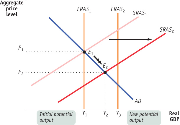
The level of potential output has risen from Y1 to Y3 and the new level of potential output is higher than the new short-
Long-Run Macroeconomic Equilibrium
Figure 12-16 combines the aggregate demand curve with both the short-run and long-run aggregate supply curves. The aggregate demand curve, AD, crosses the short-run aggregate supply curve, SRAS, at ELR. Here we assume that enough time has elapsed that the economy is also on the long-run aggregate supply curve, LRAS. As a result, ELR is at the intersection of all three curves—SRAS, LRAS, and AD. So short-run equilibrium aggregate output is equal to potential output, YP. Such a situation, in which the point of short-run macroeconomic equilibrium is on the long-run aggregate supply curve, is known as long-run macroeconomic equilibrium.
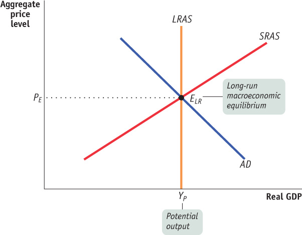
The economy is in long-run macroeconomic equilibrium when the point of short-run macroeconomic equilibrium is on the long-run aggregate supply curve.
Demand Shocks To see the significance of long-run macroeconomic equilibrium, let’s consider what happens if a demand shock moves the economy away from long-run macroeconomic equilibrium. In Figure 12-17, we assume that the initial aggregate demand curve is AD1 and the initial short-run aggregate supply curve is SRAS1. So the initial macroeconomic equilibrium is at E1, which lies on the long-run aggregate supply curve, LRAS. The economy, then, starts from a point of short-run and long-run macroeconomic equilibrium, and short-run equilibrium aggregate output equals potential output at Y1.
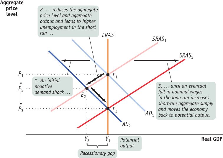
Now suppose that for some reason—such as a sudden worsening of business and consumer expectations—aggregate demand falls and the aggregate demand curve shifts leftward to AD2. This results in a lower equilibrium aggregate price level at P2 and a lower equilibrium aggregate output level at Y2 as the economy settles in the short run at E2. The short-run effect of such a fall in aggregate demand is what the Canadian economy experienced during the Great Depression and in the recent recession of 2008-2009: a falling aggregate price level and falling aggregate output.
Aggregate output in this new short-run equilibrium, E2, is below potential output. When this happens, the economy faces a recessionary gap. A recessionary gap inflicts a great deal of pain because it corresponds to high unemployment. The large recessionary gap that had opened up in Canada by 1933 caused intense social and political turmoil. And the devastating recessionary gap that opened up in Germany at the same time played an important role in Hitler’s rise to power.
There is a recessionary gap when aggregate output is below potential output.
But this isn’t the end of the story. In the face of high unemployment, nominal wages eventually fall, as do any other sticky prices, ultimately leading producers to increase output. As a result, a recessionary gap causes the short-run aggregate supply curve to gradually shift to the right over time. This process continues until SRAS1 reaches its new position at SRAS2, bringing the economy to equilibrium at E3, where AD2, SRAS2, and LRAS all intersect. At E3, the economy is back in long-run macroeconomic equilibrium; it is back at potential output Y1 but at a lower aggregate price level, P3, reflecting a long-run fall in the aggregate price level. In the end, the economy is self-correcting in the long run.
WHERE’S THE DEFLATION?
The AD-AS model says that either a negative demand shock or a positive supply shock should lead to a fall in the aggregate price level—that is, deflation. However, since 1945, an actual fall in the aggregate price level has been a rare occurrence in Canada. Similarly, most other countries have had little or no experience with deflation. Japan, which experienced sustained mild deflation in the late 1990s and the early part of the next decade, is the big (and much discussed) exception. What happened to deflation?
The basic answer is that economic fluctuations since World War II have largely taken place around a long-run inflationary trend. Before the war, it was common for prices to fall during recessions, but since then negative demand shocks have largely been reflected in a decline in the rate of inflation rather than an actual fall in prices. For example, the annualized inflation rate fell from 11.3% in January 1982 (the beginning of the recession in the early 1980s) to 5.01% in September 1983 (the end of the recession), but never fell below zero.
All of this changed following the recession of 1990-1991. The annualized inflation rate actually rose from 5.5% in January 1990 to 6.91% in January before falling to 3.75% in December 1991. Then the annual rate of inflation fell below 2% for most months during 1992 to 1994. In May, October, and November of 1994, the CPI actually declined on an annual basis—Canada experienced deflation.
Canada experienced deflation again during the recession of 2008-2009. The negative demand shock that followed the 2007-2008 U.S. financial crisis was so severe that, from June 2009 to September 2009, consumer prices in Canada indeed fell, compared to the same period in the previous year. But the deflationary period didn’t last long. Starting in October 2009, prices again rose, at a rate of between 1% and 3% per year.
Figure 12-18 shows the results of an increase in aggregate demand. In the short run, a rightward shift in aggregate demand leads to a rise in both aggregate price level and aggregate output. Since the short-run equilibrium level of output, Y2, is above the level of potential output, the economy is said to be in an inflationary gap. Such a gap lowers unemployment and puts upward pressure on nominal wages. This, in the longer term, shifts the short-run aggregate supply curve up to the left. When the economy settles into its new long-run equilibrium, E3, output falls back to potential output and the aggregate price level increases farther to P3. Just as in the case of a reduction in aggregate demand, the economy corrects itself.
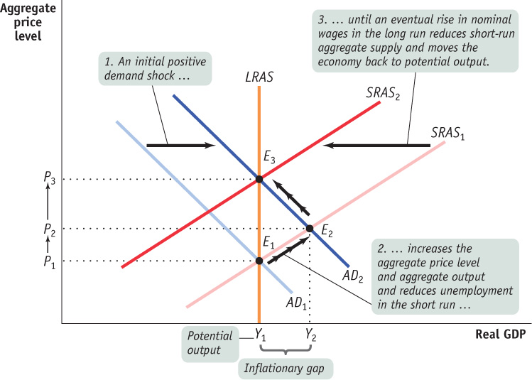
There is an inflationary gap when aggregate output is above potential output.
To summarize the analysis of how the economy responds to recessionary and inflationary gaps, we can focus on the output gap, the percentage difference between actual aggregate output and potential output. The output gap is calculated as follows:

The output gap is the percentage difference between actual aggregate output and potential output.
Our analysis says that the output gap always tends toward zero.
If there is a recessionary gap, so that the output gap is negative, nominal wages eventually fall, moving the economy back to potential output and bringing the output gap back to zero. If there is an inflationary gap, so that the output gap is positive, nominal wages eventually rise, also moving the economy back to potential output and again bringing the output gap back to zero. So in the long run the economy is self-correcting: shocks to aggregate demand affect aggregate output in the short run but not in the long run.
The economy is self-correcting when shocks to aggregate demand affect aggregate output in the short run, but not the long run.
Supply Shocks We have examined the long-run adjustment following a demand shock, but what happens if there is supply shock that moves the economy away from long-run macroeconomic equilibrium? Let’s continue with the example of the simultaneous shifts in both the SRAS and LRAS curves discussed earlier.
The short-run and long-run effects of an increase in productivity are shown in Figure 12-19. The initial equilibrium is at E1, with aggregate price level P1 and aggregate output Y1. The rise in productivity leads to a rightward shift in both the short-run and long-run aggregate supply curves to SRAS2 and LRAS2, respectively. This results in a lower equilibrium aggregate price level at P2 and a higher equilibrium level of aggregate output at Y2 as the economy settles in the short-run at E2. Although the short-run equilibrium level of aggregate output has increased, it is now below the new level of potential output, Y3. In the longer term, we will observe a fall in nominal wages and other sticky prices. This will further increase output as it causes the short-run aggregate supply curve to gradually shift to the right over time. This process continues until SRAS reaches its long-run position, SRAS3, where AD, SRAS3, and LRAS2 all intersect. At the new long-run equilibrium, E3, the economy finds its aggregate output has moved to the new level of potential output Y3 and the aggregate price level has fallen farther to P3. Once again, the economy is self-correcting in the long-run.
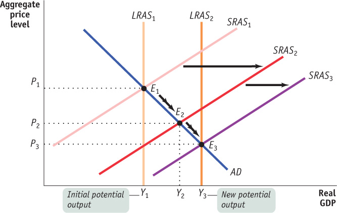
An increase in productivity shifts both the short-run and long-run aggregate supply curves to the right. The economy moves from E1 to E2 in the short-run. The aggregate price level falls from P1 to P2, and aggregate output rises from Y1 to Y2.
SUPPLY SHOCKS VERSUS DEMAND SHOCKS IN PRACTICE
How often do supply shocks and demand shocks, respectively, cause recessions? The verdict of most, though not all, macroeconomists is that recessions are mainly caused by demand shocks. But when a negative supply shock does happen, the resulting recession tends to be particularly severe.
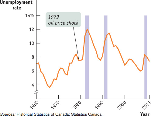
Let’s get specific. Canada has experienced three recessions in the past 50 years: one in 1982-1983, one in 1990-1991, and the third in 2008-2009. The first recession was caused by a supply shock—political turmoil in the Middle East in the late 1970s led to disruption of oil supplies, and oil prices skyrocketed. This recession was the only one to show the distinctive combination of falling aggregate output and a surge in the price level, or in a word, stagflation. Some of the highest unemployment rates since 1960, in fact since the Great Depression, came following this big negative supply shock. In contrast, the last two recessions were caused by demand shocks, and although unpleasant, they were not nearly as bad as the recession in the early 1980s. Although unemployment rates were up, the Canadian economy did not experience a significantly higher rate of inflation. Figure 12-20 shows Canada’s unemployment rate since 1960, with the date of the oil price shock in the late 1970s indicated and the periods of recession highlighted in purple.
There’s a reason the aftermath of a supply shock tends to be particularly severe for the economy: macroeconomic policy has a much harder time dealing with supply shocks than with demand shocks. For example, the reason the Bank of Canada was having a hard time in 2008, as described in the opening story, was the fact that in early 2008 the Canadian economy was hit by an adverse supply shock (although it was also facing an adverse demand shock). We’ll see in a moment why supply shocks present such a problem.

Quick Review
The AD-AS model is used to study economic fluctuations.
Short-run macroeconomic equilibrium occurs at the intersection of the short-run aggregate supply and aggregate demand curves. This determines the short-run equilibrium aggregate price level and the level of short-run equilibrium aggregate output.
A demand shock, a shift of the AD curve, causes the aggregate price level and aggregate output to move in the same direction. A supply shock, a shift of the SRAS curve, causes them to move in opposite directions. Stagflation is the consequence of a negative supply shock.
A fall in nominal wages occurs in response to a recessionary gap, and a rise in nominal wages occurs in response to an inflationary gap. Both move the economy to long-run macroeconomic equilibrium, where the AD, SRAS, and LRAS curves intersect.
The output gap always tends toward zero because the economy is self-correcting in the long run.
Check Your Understanding 12-3
CHECK YOUR UNDERSTANDING 12-3
Question 12.4
Describe the short-run effects of each of the following shocks on the aggregate price level and on aggregate output.
The government sharply increases the minimum wage, raising the wages of many workers.
Solar energy firms launch a major program of investment spending.
The federal government raises taxes and cuts spending.
Severe weather destroys crops around the world.
An increase in the minimum wage raises the nominal wage and, as a result, shifts the short-run aggregate supply curve to the left. As a result of this negative supply shock, the aggregate price level rises and aggregate output falls.
Increased investment spending shifts the aggregate demand curve to the right. As a result of this positive demand shock, both the aggregate price level and aggregate output rise.
An increase in taxes and a reduction in government spending both result in negative demand shocks, shifting the aggregate demand curve to the left. As a result, both the aggregate price level and aggregate output fall.
This is a negative supply shock, shifting the short-run aggregate supply curve to the left. As a result, the aggregate price level rises and aggregate output falls.
Question 12.5
A rise in productivity increases potential output, but some worry that demand for the additional output will be insufficient even in the long run. How would you respond?
As the rise in productivity increases potential output, the long-run aggregate supply curve shifts to the right. If, in the short run, there is now a recessionary gap (aggregate output is less than potential output), nominal wages will fall, shifting the short-run aggregate supply curve to the right. This results in a fall in the aggregate price level and a rise in aggregate output. As prices fall, we move along the aggregate demand curve due to the wealth and interest rate effects of a change in the aggregate price level. Eventually, as long-run macroeconomic equilibrium is reestablished, aggregate output will rise to be equal to potential output.