15.4 Money, Output, and Prices in the Long Run
Through its expansionary and contractionary effects, monetary policy is generally the policy tool of choice to help stabilize the economy. However, not all actions by central banks are productive. In particular, as we’ll see in the next chapter, central banks sometimes print money not to fight a recessionary gap but to help the government pay its bills, an action that typically destabilizes the economy.
What happens when a change in the money supply pushes the economy away from, rather than toward, long-
Short-Run and Long-Run Effects of an Increase in the Money Supply
To analyze the long-
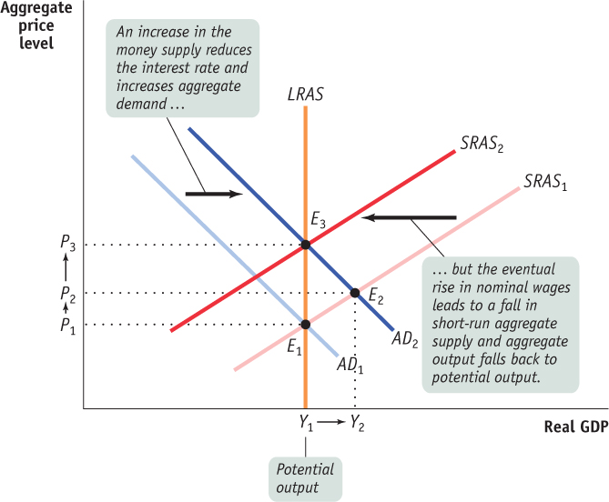
Here, the economy begins at E1, a point of short-
The economy reaches a new short-
Figure 15-13 shows the short-
Now suppose there is an increase in the money supply. Other things equal, an increase in the money supply reduces the interest rate, which increases investment spending, which leads to a further rise in consumer spending, and so on. So an increase in the money supply increases the quantity of goods and services demanded, shifting the AD curve rightward, to AD2. In the short run, the economy moves to a new short-
But the aggregate output level, Y2, is above potential output. As a result, in the longer term, nominal wages will rise over time, causing the short-
We won’t describe the effects of a monetary contraction in detail, but the same logic applies. In the short run, a fall in the money supply leads to a fall in aggregate output as the economy moves down the short-
Monetary Neutrality
How much does a change in the money supply change the aggregate price level in the long run? The answer is that a change in the money supply leads to an equal proportional change in the aggregate price level in the long run. For example, if the money supply falls 25%, the aggregate price level falls 25% in the long run; if the money supply rises 50%, the aggregate price level rises 50% in the long run.
How do we know this? Consider the following thought experiment: Suppose all prices in the economy—
We can state this argument in reverse: If the economy starts out in long-
According to the concept of monetary neutrality, changes in the money supply have no real effects on the economy.
This analysis demonstrates the concept known as monetary neutrality, in which changes in the money supply have no real effects on the economy. In the long run, the only effect of an increase in the money supply is to raise the aggregate price level by an equal percentage. Economists argue that money is neutral in the long run.
This is, however, a good time to recall the dictum of John Maynard Keynes: “In the long run we are all dead.” In the long run, changes in the money supply don’t have any effect on real GDP, interest rates, or anything else except the price level. But it would be foolish to conclude from this that the BOC is irrelevant. Monetary policy does have powerful real effects on the economy in the short run, often making the difference between recession and expansion. And that matters a lot for society’s welfare.
Changes in the Money Supply and the Interest Rate in the Long Run
In the short run, an increase in the money supply leads to a fall in the interest rate, and a decrease in the money supply leads to a rise in the interest rate. In the long run, however, changes in the money supply don’t affect the interest rate.
 to
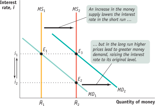
to  pushes the interest rate down from i1 to i2 and the economy moves to E2, a short-run equilibrium. In the long run, however, the aggregate price level rises in proportion to the increase in the money supply, leading to an increase in money demand at any given interest rate in proportion to the increase in the aggregate price level, as shown by the shift from MD1 to MD2. The result is that the quantity of money demanded at any given interest rate rises by the same amount as the quantity of money supplied. The economy moves to long-run equilibrium at E3 and the interest rate returns to i1.
Figure 15-14 shows why. It shows the money supply curve and the money demand curve before and after the BOC increases the money supply. We assume that the economy is initially at E1, in long-run macroeconomic equilibrium at potential output, and with money supply
. The initial equilibrium interest rate, determined by the intersection of the money demand curve MD1 and the money supply curve MS1, is i1.
Now suppose the money supply increases from
to
. In the short run, the economy moves from E1 to E2 and the interest rate falls from i1 to i2. Over time, however, the aggregate price level rises, and this raises money demand, shifting the money demand curve rightward from MD1 to MD2. The economy moves to a new long-run equilibrium at E3, and the interest rate rises to its original level at i1.
And it turns out that the long-run equilibrium nominal interest rate is the original interest rate, i1. We know this for two reasons. First, due to monetary neutrality, in the long run the aggregate price level rises by the same proportion as the money supply; so if the money supply rises by, say, 50%, the price level will also rise by 50%. Second, the demand for money is, other things equal, proportional to the aggregate price level. So a 50% increase in the money supply raises the aggregate price level by 50%, which increases the quantity of money demanded at any given interest rate by 50%. As a result, the quantity of money demanded at the initial interest rate, i1, rises exactly as much as the money supply—so that i1 is still the equilibrium interest rate. In the long run, then, changes in the money supply do not affect the interest rate.
INTERNATIONAL EVIDENCE OF MONETARY NEUTRALITY
These days monetary policy is quite similar among wealthy countries. Each major nation (or, in the case of the euro, the euro area) has a central bank that is insulated from political pressure. All of these central banks try to keep the aggregate price level roughly stable, which usually means inflation of at most 2% to 3% per year.
But if we look at a longer period and a wider group of countries, we see large differences in the growth of the money supply. Between 1970 and the present, the money supply rose only a few percent per year in some countries, such as Canada, Switzerland, and the United States, but rose much more rapidly in some poorer countries, such as South Africa. These differences allow us to see whether it is really true that increases in the money supply lead, in the long run, to equal percent rises in the aggregate price level.
Figure 15-15 shows the annual percentage increases in the money supply and average annual increases in the aggregate price level—that is, the average rate of inflation—for a sample of countries during the period 1970–2010, with each point representing a country. If the relationship between increases in the money supply and changes in the aggregate price level were exact, the points would lie precisely on a 45-degree line. In fact, the relationship isn’t exact, because other factors besides money affect the aggregate price level in the short-run. But the scatter of points clearly lies close to a 45-degree line, showing a more or less proportional relationship between money and the aggregate price level. That is, the data support the concept of monetary neutrality in the long run.
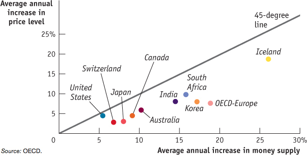
Source: OECD.

Quick Review
According to the concept of monetary neutrality, changes in the money supply do not affect real GDP, only the aggregate price level. Economists believe that money is neutral in the long run.
In the long run, the equilibrium interest rate in the economy is unaffected by changes in the money supply.
Check Your Understanding 15-4
CHECK YOUR UNDERSTANDING 15-4
Question 15.8
Assume the central bank increases the quantity of money by 25%, even though the economy is initially in both short-run and long-run macroeconomic equilibrium. Describe the effects, in the short run and in the long run (giving numbers where possible), on the following.
Aggregate output
Aggregate price level
Interest rate
Aggregate output rises in the short run, then falls back to equal potential output in the long run.
The aggregate price level rises in the short run, but by less than 25%. It rises further in the long run, for a total increase of 25%.
The interest rate falls in the short run, then rises back to its original level in the long run.
Question 15.9
Why does monetary policy affect the economy in the short run but not in the long run?
In the short run, a change in the interest rate alters the economy because it affects investment spending, which in turn affects aggregate demand and real GDP through the multiplier process. However, in the long run, changes in consumer spending and investment spending will eventually result in changes in nominal wages and the nominal prices of other factors of production. For example, an expansionary monetary policy will eventually cause a rise in factor prices; a contractionary policy will eventually cause a fall in factor prices. In response, the short-run aggregate supply curve will shift to move the economy back to long-run equilibrium. So in the long run monetary policy has no effect on the economy.
Was Quantitative Easing A Good Choice?

Usually, central banks set the price of money and attempt to steer the economy using their policy interest rate. But when the overnight interest rate is close to zero percent, or equal to it, the impact of the central bank’s target for the overnight rate on the economy becomes limited. In such circumstances, if the central bank wishes to affect the price of money to stimulate the economy it can turn to quantitative easing (QE).
With quantitative easing, the central bank “creates new money,” which it then uses to buy assets in the domestic economy: government bonds, stocks, corporate bonds, assets from financial institutions, and so on. When the central bank buys long-term bonds their prices rise, causing their interest rates to fall. Lower interest rates stimulate spending, which should help to pull the economy out of its slump. Thus does the central bank hope to add further stimulus to the economy using QE.
Or so the theory goes. QE can be tricky—if not outright dangerous. A central bank that uses QE might lose money on the assets it buys. Even worse, if the central bank creates too much money, or does not remove the money quickly enough when the economy recovers, then the currency will be devalued by inflation. Furthermore, the fact that QE is being used at all may ruin confidence in an economy rather than build it. According to Financial Times economics editor Chris Giles, “This is why central banks cannot use QE willy-nilly, but if you are not aggressive enough QE simply will not work to change other interest rates in the economy and stimulate demand. The trouble is, because the policy is unorthodox and the situation is dramatic no one knows how much QE is too much and how much is not enough.”
Unfortunately, so far QE has created a questionable degree of stimulus where it has been used—United States, England, Japan, and the eurozone—and of course, has drawn criticism in each of these places. Indeed, no central bank really does seem to know how much is enough—the U.S., for instance, has rolled out three (or perhaps four) rounds of QE.
Canada’s relatively strong economy has meant that the Bank of Canada has not needed to adopt QE. But have we benefitted from QE nonetheless? To an extent, yes. Since the U.S. has used QE to stimulate its economy and create jobs, there is a corresponding increase in demand for exports from nations such as Canada, which is to our benefit. On the other hand, using this expansionary monetary policy puts downward pressure on the U.S. dollar exchange rate, so the Canadian dollar appreciates, which is to our detriment.
Interestingly, Camilla Sutton, the Bank of Nova Scotia’s chief currency strategist (pictured here), devised a way that Canadian investors could profit from QE. She calculated that in 2012, investors could have made about a 5.5 percent profit without using any leverage. Her strategy is to sell currencies of countries that are engaging in QE and buy currencies of those that are not. In doing so, the investor is betting that the relative exchange rate will move against countries engaging in QE because they are creating too much money. So it seems the laws of economics do hold: if a central bank prints too much money, then it creates inflation and lowers the exchange rate. And better yet, it seems Canadians might be able to profit from it.
QUESTIONS FOR THOUGHT
Question 15.10
Why do central banks have difficulty using their policy interest rates to stimulate the economy when these rates are at or near zero?
Question 15.11
How does quantitative easing (QE) help the central bank to stimulate the economy?
Question 15.12
What risks does adopting QE bring to an economy?
Question 15.13
What risks does not adopting QE bring to an economy, when a major trading partner has adopted QE?