The Income–Expenditure Model
Earlier in this chapter, we described how autonomous changes in spending—
Before we begin, let’s quickly recap the assumptions underlying the multiplier process.
Changes in overall spending lead to changes in aggregate output. We assume that producers are willing to supply additional output at a fixed price level. As a result, changes in spending translate into changes in output rather than moves of the overall price level up or down. A fixed aggregate price level also implies that there is no difference between nominal GDP and real GDP. So we can use the two terms interchangeably in this chapter.
The interest rate is fixed. We’ll take the interest rate as predetermined and unaffected by the factors we analyze in the model. As in the case of the aggregate price level, what we’re really doing here is leaving the determinants of the interest rate outside the model. As we’ll see, the model can still be used to study the effects of a change in the interest rate.
Taxes, government transfers, and government purchases are all zero.
Exports and imports are both zero.
In all subsequent chapters, we will drop the assumption that the aggregate price level is fixed. The Chapter 28 appendix addresses how taxes affect the multiplier process. We’ll explain how the interest rate is determined in Chapter 30 and bring foreign trade back into the picture in Chapter 34.
Planned Aggregate Spending and Real GDP
In an economy with no government and no foreign trade, there are only two sources of aggregate spending: consumer spending, C, and investment spending, I. And since we assume that there are no taxes or transfers, aggregate disposable income is equal to GDP (which, since the aggregate price level is fixed, is the same as real GDP): the total value of final sales of goods and services ultimately accrues to households as income. So in this highly simplified economy, there are two basic equations of national income accounting:
As we learned earlier in this chapter, the aggregate consumption function shows the relationship between disposable income and consumer spending. Let’s continue to assume that the aggregate consumption function is of the same form as in Equation 26-

In our simplified model, we will also assume planned investment spending, IPlanned, is fixed.
We need one more concept before putting the model together: planned aggregate spending, the total amount of planned spending in the economy. Unlike firms, households don’t take unintended actions like unplanned inventory investment. So planned aggregate spending is equal to the sum of consumer spending and planned investment spending. We denote planned aggregate spending by AEPlanned, so:
Planned aggregate spending is the total amount of planned spending in the economy.

The level of planned aggregate spending in a given year depends on the level of real GDP in that year. To see why, let’s look at a specific example, shown in Table 26-2. We assume that the aggregate consumption function is:

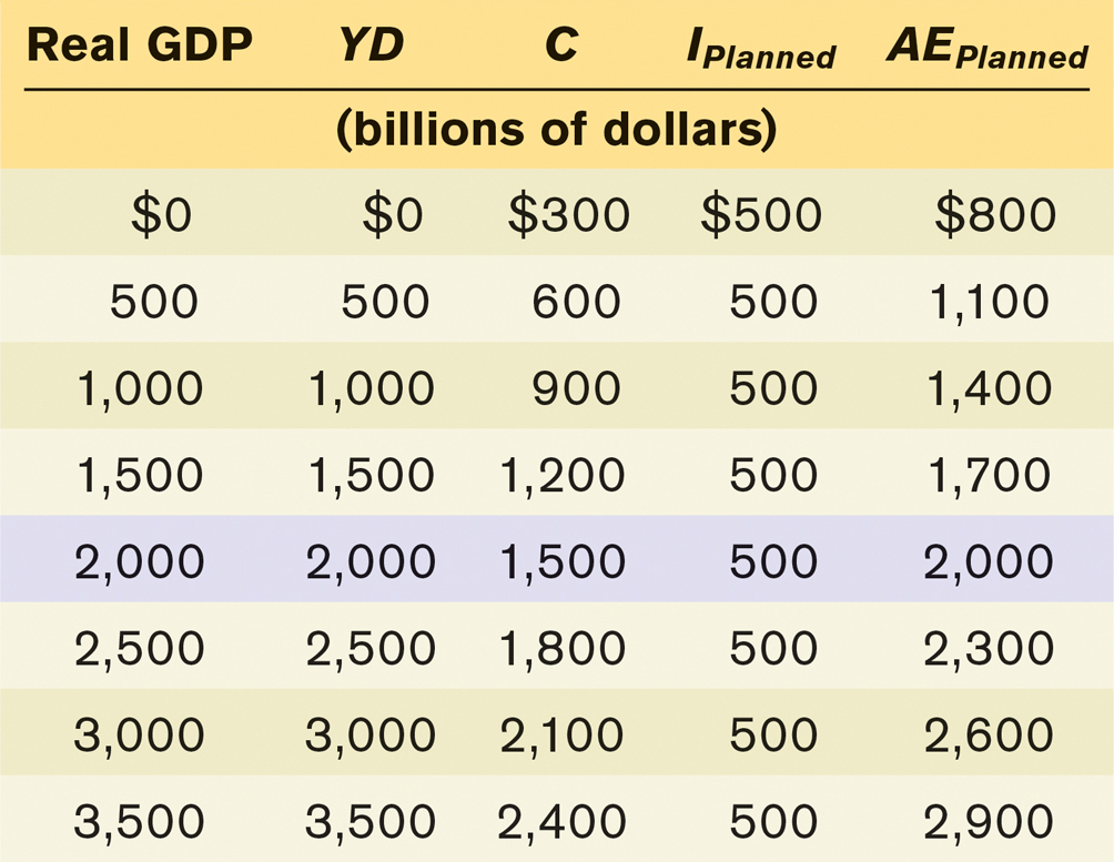
Real GDP, YD, C, IPlanned, and AEPlanned are all measured in billions of dollars, and we assume that the level of planned investment, IPlanned, is fixed at $500 billion per year. The first column shows possible levels of real GDP. The second column shows disposable income, YD, which in our simplified model is equal to real GDP. The third column shows consumer spending, C, equal to $300 billion plus 0.6 times disposable income, YD. The fourth column shows planned investment spending, IPlanned, which we have assumed is $500 billion regardless of the level of real GDP. Finally, the last column shows planned aggregate spending, AEPlanned, the sum of aggregate consumer spending, C, and planned investment spending, IPlanned. (To economize on notation, we’ll assume that it is understood from now on that all the variables in Table 26-2 are measured in billions of dollars per year.) As you can see, a higher level of real GDP leads to a higher level of disposable income: every 500 increase in real GDP raises YD by 500, which in turn raises C by 500 × 0.6 = 300 and AEPlanned by 300.
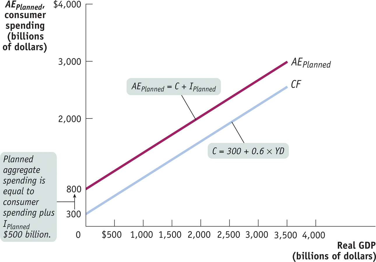
Figure 26-9 illustrates the information in Table 26-2 graphically. Real GDP is measured on the horizontal axis. CF is the aggregate consumption function; it shows how consumer spending depends on real GDP. AEPlanned, the planned aggregate spending line, corresponds to the aggregate consumption function shifted up by 500 (the amount of IPlanned). It shows how planned aggregate spending depends on real GDP. Both lines have a slope of 0.6, equal to MPC, the marginal propensity to consume.
But this isn’t the end of the story. Table 26-2 reveals that real GDP equals planned aggregate spending, AEPlanned, only when the level of real GDP is at 2,000. Real GDP does not equal AEPlanned at any other level. Is that possible? Didn’t we learn in Chapter 22, with the circular-
But as we’ll see in the next section, the economy moves over time to a situation in which there is no unplanned inventory investment, a situation called income–
Income–Expenditure Equilibrium
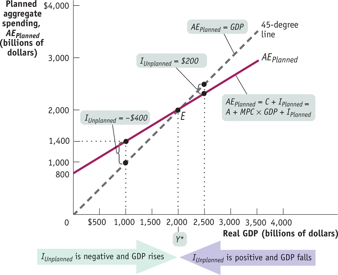
For all but one value of real GDP shown in Table 26-2, real GDP is either more or less than AEPlanned, the sum of consumer spending and planned investment spending. For example, when real GDP is 1,000, consumer spending, C, is 900 and planned investment spending is 500, making planned aggregate spending 1,400. This is 400 more than the corresponding level of real GDP. Now consider what happens when real GDP is 2,500; consumer spending, C, is 1,800 and planned investment spending is 500, making planned aggregate spending only 2,300, 200 less than real GDP.
As we’ve just explained, planned aggregate spending can be different from real GDP only if there is unplanned inventory investment, IUnplanned, in the economy. Let’s examine Table 26-3, which includes the numbers for real GDP and for planned aggregate spending from Table 26-2. It also includes the levels of unplanned inventory investment, IUnplanned, that each combination of real GDP and planned aggregate spending implies. For example, if real GDP is 2,500, planned aggregate spending is only 2,300. This 200 excess of real GDP over AEPlanned must consist of positive unplanned inventory investment. This can happen only if firms have overestimated sales and produced too much, leading to unintended additions to inventories. More generally, any level of real GDP in excess of 2,000 corresponds to a situation in which firms are producing more than consumers and other firms want to purchase, creating an unintended increase in inventories.
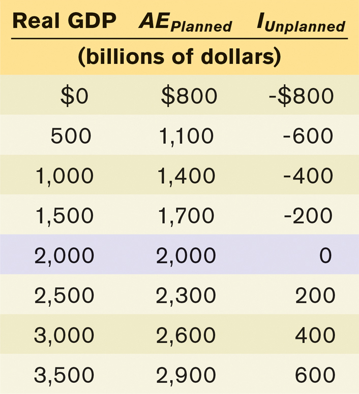
Conversely, a level of real GDP below 2,000 implies that planned aggregate spending is greater than real GDP. For example, when real GDP is 1,000, planned aggregate spending is much larger, at 1,400. The 400 excess of AEPlanned over real GDP corresponds to negative unplanned inventory investment equal to −400. More generally, any level of real GDP below 2,000 implies that firms have underestimated sales, leading to a negative level of unplanned inventory investment in the economy.
By putting together Equations 26-

So whenever real GDP exceeds AEPlanned, IUnplanned is positive; whenever real GDP is less than AEPlanned, IUnplanned is negative.
But firms will act to correct their mistakes. We’ve assumed that they don’t change their prices, but they can adjust their output. Specifically, they will reduce production if they have experienced an unintended rise in inventories or increase production if they have experienced an unintended fall in inventories. And these responses will eventually eliminate the unanticipated changes in inventories and move the economy to a point at which real GDP is equal to planned aggregate spending.
Staying with our example, if real GDP is 1,000, negative unplanned inventory investment will lead firms to increase production, leading to a rise in real GDP. In fact, this will happen whenever real GDP is less than 2,000—
The economy is in income–
The only situation in which firms won’t have an incentive to change output in the next period is when aggregate output, measured by real GDP, is equal to planned aggregate spending in the current period, an outcome known as income–
Income–
Figure 26-10 illustrates the concept of income–
This line allows us to easily spot the point of income–
Now consider what happens if the economy isn’t in income–
The Keynesian cross diagram identifies income–
The type of diagram shown in Figure 26-10, which identifies income–
The Multiplier Process and Inventory Adjustment
We’ve just learned about a very important feature of the macroeconomy: when planned spending by households and firms does not equal the current aggregate output by firms, this difference shows up in changes in inventories. The response of firms to those inventory changes moves real GDP over time to the point at which real GDP and planned aggregate spending are equal. That’s why, as we mentioned earlier, changes in inventories are considered a leading indicator of future economic activity.
Now that we understand how real GDP moves to achieve income–
In our simple model there are only two possible sources of a shift of the planned aggregate spending line: a change in planned investment spending, IPlanned, or a shift of the aggregate consumption function, CF. For example, a change in IPlanned can occur because of a change in the interest rate. (Remember, we’re assuming that the interest rate is fixed by factors that are outside the model. But we can still ask what happens when the interest rate changes.) A shift of the aggregate consumption function (that is, a change in its vertical intercept, A) can occur because of a change in aggregate wealth—
Recall from earlier in this chapter that an autonomous change in planned aggregate spending is a change in the desired level of spending by firms, households, and government at any given level of real GDP (although we’ve assumed away the government for the time being). How does an autonomous change in planned aggregate spending affect real GDP in income–
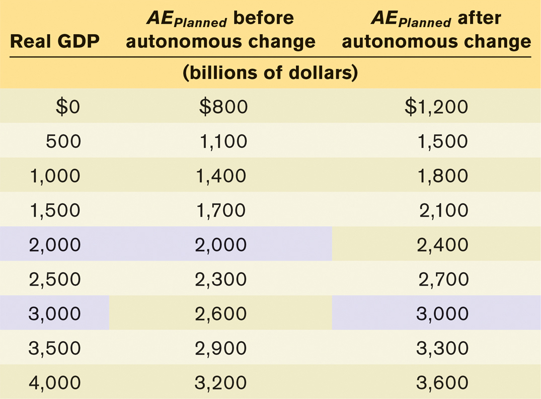
Table 26-4 and Figure 26-11 start from the same numerical example we used in Table 26-3 and Figure 26-10. They also show the effect of an autonomous increase in planned aggregate spending of 400— is 2,000. The autonomous rise in planned aggregate spending shifts the planned aggregate spending line up, leading to a new income–
 is 3,000.
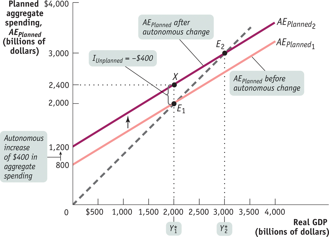 , equal to 2,000. An autonomous increase in AEPlanned of 400 shifts the planned aggregate spending line upward by 400. The economy is no longer in income–, equal to 3,000.
The fact that the rise in income–
We can examine in detail what underlies the multistage multiplier process by looking more closely at Figure 26-11. First, starting from E1, the autonomous increase in planned aggregate spending leads to a gap between planned aggregate spending and real GDP. This is represented by the vertical distance between X, at 2,400, and E1, at 2,000. This gap illustrates an unplanned fall in inventory investment: IUnplanned = − 400. Firms respond by increasing production, leading to a rise in real GDP from . The rise in real GDP translates into an increase in disposable income, YD. That’s the first stage in the chain reaction. But it doesn’t stop there—
We can summarize these results in an equation, where ΔAAEPlanned represents the autonomous change in AEPlanned, and  , the subsequent change in income–

Recalling that the multiplier, 1/(1 − MPC), is greater than 1, Equation 26-.
The Paradox of Thrift You may recall that in Chapter 21 we mentioned the paradox of thrift to illustrate the fact that in macroeconomics the outcome of many individual actions can generate a result that is different from and worse than the simple sum of those individual actions. In the paradox of thrift, households and firms cut their spending in anticipation of future tough economic times. These actions depress the economy, leaving households and firms worse off than if they hadn’t acted virtuously to prepare for tough times. It is called a paradox because what’s usually “good” (saving to provide for your family in hard times) is “bad” (because it can make everyone worse off).
Using the multiplier, we can now see exactly how this scenario unfolds. Suppose that there is a slump in consumer spending or investment spending, or both, just like the slump in residential construction investment spending leading up to the 2007–
Conversely, prodigal behavior is rewarded: if consumers or producers increase their spending, the resulting multiplier process makes the increase in income–
It’s important to realize that our result that the multiplier is equal to 1/(1 − MPC) depends on the simplifying assumption that there are no taxes or transfers, so that disposable income is equal to real GDP. In the appendix to Chapter 28, we’ll bring taxes into the picture, which makes the expression for the multiplier more complicated and the multiplier itself smaller. But the general principle we have just learned—

As we noted earlier in this chapter, declines in planned investment spending are usually the major factor causing recessions, because historically they have been the most common source of autonomous reductions in aggregate spending. The tendency of the consumption function to shift upward over time, which we pointed out earlier in the Economics in Action, “Famous First Forecasting Failures,” means that autonomous changes in both planned investment spending and consumer spending play important roles in expansions. But regardless of the source, there are multiplier effects in the economy that magnify the size of the initial change in aggregate spending.
ECONOMICS in Action: Inventories and the End of a Recession
Inventories and the End of a Recession
Avery clear example of the role of inventories in the multiplier process took place in late 2001, as that year’s recession came to an end. The driving force behind the recession was a slump in business investment spending. It took several years before investment spending bounced back in the form of a housing boom. Still, the economy did start to recover in late 2001, largely because of an increase in consumer spending—
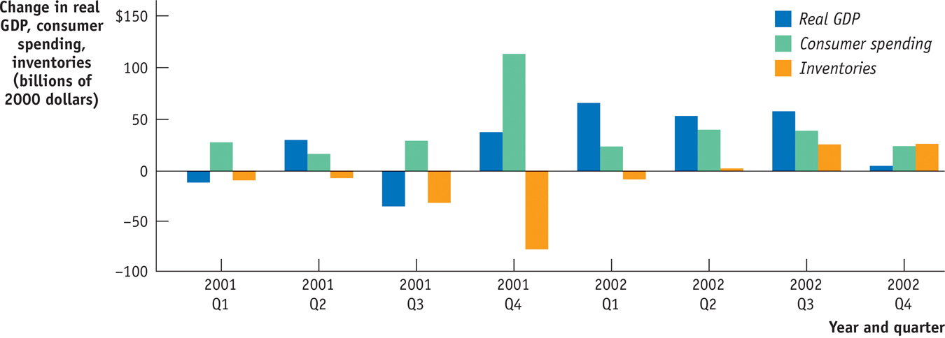
Initially, this increase in consumer spending caught manufacturers by surprise. Figure 26-12 shows changes in real GDP, real consumer spending, and real inventories in each quarter of 2001 and 2002. Notice the surge in consumer spending in the fourth quarter of 2001. It didn’t lead to a lot of GDP growth because it was offset by a plunge in inventories. But in the first quarter of 2002 producers greatly increased their production, leading to a jump in real GDP.
Quick Review
The economy is in income–
expenditure equilibrium when planned aggregate spending is equal to real GDP. At any output level greater than income–
expenditure equilibrium GDP, real GDP exceeds planned aggregate spending and inventories are rising. At any lower output level, real GDP falls short of planned aggregate spending and inventories are falling. After an autonomous change in planned aggregate spending, the economy moves to a new income–
expenditure equilibrium through the inventory adjustment process, as illustrated by the Keynesian cross. Because of the multiplier effect, the change in income– expenditure equilibrium GDP is a multiple of the autonomous change in aggregate spending.
26-4
Question 11.9
Although economists believe that recessions typically begin as slumps in investment spending, they also believe that consumer spending eventually slumps during a recession. Explain why.
Question 11.10
Use a diagram like Figure 26-10 to show what happens when there is an autonomous fall in planned aggregate spending. Describe how the economy adjusts to a new income–
expenditure equilibrium. Suppose Y* is originally $500 billion, the autonomous reduction in planned aggregate spending is $300 million ($0.3 billion), and MPC = 0.5. Calculate Y* after such a change.
Solutions appear at back of book.
What’s Good for America Is Good for GM
In 2009, with the economy in a steep nose-
General Motors—

By 2009 the fate of GM and the fate of America seemed less intertwined. Still, the case for the bailout rested crucially on the belief that GM’s problems weren’t entirely self-
On the face of it, this interdependence wasn’t entirely obvious: the 2007–
Did saving GM justify the bailout? The company’s recovery meant that taxpayers got most of their money back—
Defenders of the bailout nonetheless declared it a success, because it resuscitated the U.S. auto industry and saved many jobs, not just in the auto companies and their suppliers, but in the many businesses whose sales depend on the incomes of workers employed in the auto industry. In the summer of 2009 the unemployment rate in Michigan, still America’s automotive heartland, rose above 14%—but it then began a rapid decline, falling to 7.4% by early 2014. Few would argue that the speedy recovery in employment in Michigan would have happened without the auto bailout.
In the end, GM bounced back because the U.S. economy as a whole recovered; what was good for America was indeed still good for General Motors. And what was good for General Motors was clearly good for Michigan—
QUESTIONS FOR THOUGHT
Question 11.11
tSay3ZTP0liTQ1ZyMS7o4jvQQz44bQr0IpL/ka73jAIYrTM0jyB4YdlBex0ODnHPe4CaavpW/SezoT1ofJT7TeZZ6vbuGfPkpF3X5bE2+iLSj/LWaQX8jGRN7fk=Why did a national slump that began with housing affect companies like General Motors?Question 11.12
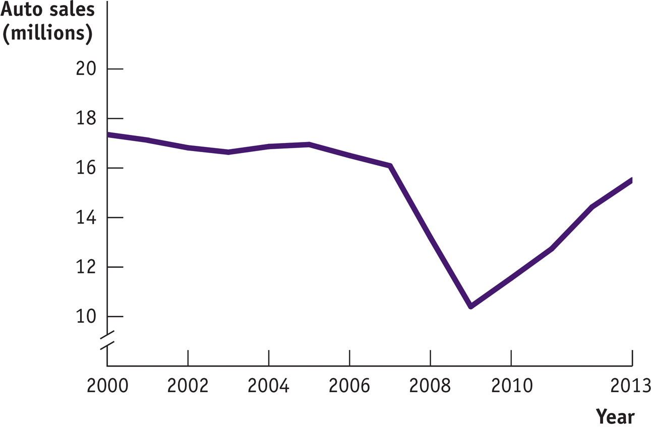
G1WYd/Rbrkzu0T1/05WNSV6Ldv6EjUI6yjA+aG94j1ThibKdJks2dxM9kuQWq67E5BM6//3n3z1N8BZJyZN2Z9kMEbzwCQW1mzumTnf+1w5t9GDto1n3Pnmy03cW1dp3ZSZFEQ==Why was it reasonable in June 2009 to predict that auto sales would improve in the near future?Question 11.13
PtQw5ct7N8cyIuAvWy0M02uN1OlmS9W2b26wyeUz2kxwiXD4QYrcv5UvU98fVip65Q+IuSkYPUt1fpygi8GUWy0NgL7OjiY/d7D7a2IxQfskTJwJ2wUssWrIc36rJw+5XkKrdvQTNyG8jGaZRSB/YEHG7yQ4vcwq7oYH1dVmv3+hQdIBdkd5N9sgyF8JEc1Y/8wXj04cqO7X/jxUplWqL6QulGDU6ruInnC9vzzEAvY2dvnYKGy5I8nDJBx54hyipMYSTWRnTTuxw/zJ14cV0R+wESMHTx+eytcXr0irG3OR4s73J19EZ0LWgw6GR5OXdUAedwrRa9DHRP41cwuFXA/mrY1qCcM94gx8+A==How does this story about General Motors help explain how a slump in housing—a relatively small part of the U.S. economy— could produce such a deep national recession?