Moderate Inflation and Disinflation
The governments of wealthy, politically stable countries, like the United States and Britain, don’t find themselves forced to print money to pay their bills. Yet over the past 40 years, both countries, along with a number of other nations, have experienced uncomfortable episodes of inflation. In the United States, the inflation rate peaked at 13% at the beginning of the 1980s. In Britain, the inflation rate reached 26% in 1975. Why did policy makers allow this to happen?
The answer, in brief, is that in the short run, policies that produce a booming economy also tend to lead to higher inflation, and policies that reduce inflation tend to depress the economy. This creates both temptations and dilemmas for governments.
First, imagine yourself as a politician facing an election in a year or two, and suppose that inflation is fairly low at the moment. You might well be tempted to pursue expansionary policies that will push the unemployment rate down as a way to please voters, even if your economic advisers warn that this will eventually lead to higher inflation. You might also be tempted to find different economic advisers who will tell you not to worry: in politics, as in ordinary life, wishful thinking often prevails over realistic analysis.
Conversely, imagine yourself as a politician in an economy suffering from inflation. Your economic advisers will probably tell you that the only way to bring inflation down is to push the economy into a recession, which will lead to temporarily higher unemployment. Are you willing to pay that price? Maybe not.
This political asymmetry—inflationary policies often produce short-term political gains, but policies to bring inflation down carry short-term political costs—explains how countries with no need to impose an inflation tax sometimes end up with serious inflation problems. For example, that 26% rate of inflation in Britain was largely the result of the British government’s decision in 1971 to pursue highly expansionary monetary and fiscal policies. Politicians disregarded warnings that these policies would be inflationary and were extremely reluctant to reverse course even when it became clear that the warnings had been correct.
But why do expansionary policies lead to inflation? To answer that question, we need to look first at the relationship between output and unemployment.
The Output Gap and the Unemployment Rate
In Chapter 27 we introduced the concept of potential output, the level of real GDP that the economy would produce once all prices had fully adjusted. Potential output typically grows steadily over time, reflecting long-run growth. However, as we learned from the aggregate demand–aggregate supply model, actual aggregate output fluctuates around potential output in the short run: a recessionary gap arises when actual aggregate output falls short of potential output; an inflationary gap arises when actual aggregate output exceeds potential output.
Recall from Chapter 27 that the percentage difference between the actual level of real GDP and potential output is called the output gap. A positive or negative output gap occurs when an economy is producing more than or less than what would be “expected” because all prices have not yet adjusted. And wages, as we’ve learned, are the prices in the labor market.
Meanwhile, we learned in Chapter 23 that the unemployment rate is composed of cyclical unemployment and natural unemployment, the portion of the unemployment rate unaffected by the business cycle. So there is a relationship between the unemployment rate and the output gap. This relationship is defined by two rules:
When actual aggregate output is equal to potential output, the actual unemployment rate is equal to the natural rate of unemployment.
When the output gap is positive (an inflationary gap), the unemployment rate is below the natural rate. When the output gap is negative (a recessionary gap), the unemployment rate is above the natural rate.
In other words, fluctuations of aggregate output around the long-run trend of potential output correspond to fluctuations of the unemployment rate around the natural rate.
This makes sense. When the economy is producing less than potential output—when the output gap is negative—it is not making full use of its productive resources. Among the resources that are not fully utilized is labor, the economy’s most important resource. So we would expect a negative output gap to be associated with unusually high unemployment. Conversely, when the economy is producing more than potential output, it is temporarily using resources at higher-than-normal rates. With this positive output gap, we would expect to see lower-than-normal unemployment.
Figure 31-4 confirms this rule. Panel (a) shows the actual and natural rates of unemployment, as estimated by the Congressional Budget Office (CBO). Panel (b) shows two series. One is cyclical unemployment: the difference between the actual unemployment rate and the CBO estimate of the natural rate of unemployment, measured on the left. The other is the CBO estimate of the output gap, measured on the right. To make the relationship clearer, the output gap series is inverted—shown upside down—so that the line goes down if actual output rises above potential output and up if actual output falls below potential output.
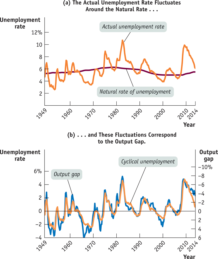
Cyclical Unemployment and the Output Gap Panel (a) shows the actual U.S. unemployment rate from 1949 through 2014, together with the Congressional Budget Office estimate of the natural rate of unemployment. The actual rate fluctuates around the natural rate, often for extended periods. Panel (b) shows cyclical unemployment—the difference between the actual unemployment rate and the natural rate of unemployment—and the output gap, also estimated by the CBO. The unemployment rate is measured on the left vertical axis, and the output gap is measured with an inverted scale on the right vertical axis. With an inverted scale, it moves in the same direction as the unemployment rate: when the output gap is positive, the actual unemployment rate is below its natural rate; when the output gap is negative, the actual unemployment rate is above its natural rate. The two series track one another closely, showing the strong relationship between the output gap and cyclical unemployment.Sources: Federal Reserve Bank of St. Louis; Congressional Budget Office.
As you can see, the two series move together quite closely, showing the strong relationship between the output gap and cyclical unemployment. Years of high cyclical unemployment, like 1982, 1992, or 2009, were also years of a strongly negative output gap. Years of low cyclical unemployment, like the late 1960s or 2000, were also years of a strongly positive output gap.
FOR INQUIRING MINDS: Okun’s Law
Although cyclical unemployment and the output gap move together, cyclical unemployment seems to move less than the output gap. For example, the output gap reached −8% in 1982, but the cyclical unemployment rate reached only 4%. This observation is the basis of an important relationship originally discovered by Arthur Okun, John F. Kennedy’s chief economic adviser.
Okun’s law is the negative relationship between the output gap and cyclical unemployment.
Modern estimates of Okun’s law—the negative relationship between the output gap and the unemployment rate—typically find that a rise in the output gap of 1 percentage point reduces the unemployment rate by about ½ of a percentage point.
For example, suppose that the natural rate of unemployment is 5.2% and that the economy is currently producing at only 98% of potential output. In that case, the output gap is −2%, and Okun’s law predicts an unemployment rate of 5.2% − ½ × (–2%) = 6.2%.
The fact that a 1% rise in output reduces the unemployment rate by only ½ of 1% may seem puzzling: you might have expected to see a one-to-one relationship between the output gap and unemployment. Doesn’t a 1% rise in aggregate output require a 1% increase in employment? And shouldn’t that take 1% off the unemployment rate?
The answer is no: there are several well-understood reasons why the relationship isn’t one-to-one. For one thing, companies often meet changes in demand in part by changing the number of hours their existing employees work. For example, a company that experiences a sudden increase in demand for its products may cope by asking (or requiring) its workers to put in longer hours, rather than by hiring more workers. Conversely, a company that sees sales drop will often reduce workers’ hours rather than lay off employees. This behavior dampens the effect of output fluctuations on the number of workers employed.
Also, the number of workers looking for jobs is affected by the availability of jobs. Suppose that the number of jobs falls by 1 million. Measured unemployment will rise by less than 1 million because some unemployed workers become discouraged and give up actively looking for work. (Recall from Chapter 23 that workers aren’t counted as unemployed unless they are actively seeking work.) Conversely, if the economy adds 1 million jobs, some people who haven’t been actively looking for work will begin doing so. As a result, measured unemployment will fall by less than 1 million.
Finally, the rate of growth of labor productivity generally accelerates during booms and slows down or even turns negative during busts. The reasons for this phenomenon are the subject of some dispute among economists. The consequence, however, is that the effects of booms and busts on the unemployment rate are dampened.
The Short-Run Phillips Curve
We’ve just seen that expansionary policies lead to a lower unemployment rate. Our next step in understanding the temptations and dilemmas facing governments is to show that there is a short-run trade-off between unemployment and inflation—lower unemployment tends to lead to higher inflation, and vice versa. The key concept is that of the Phillips curve.
The origins of this concept lie in a famous 1958 paper by the New Zealand–born economist A. W. H. Phillips. Looking at historical data for Britain, he found that when the unemployment rate was high, the wage rate tended to fall, and when the unemployment rate was low, the wage rate tended to rise. Using data from Britain, the United States, and elsewhere, other economists soon found a similar apparent relationship between the unemployment rate and the rate of inflation—that is, the rate of change in the aggregate price level. For example, Figure 31-5 shows the U.S. unemployment rate and the rate of consumer price inflation over each subsequent year from 1955 to 1968, with each dot representing one year’s data.
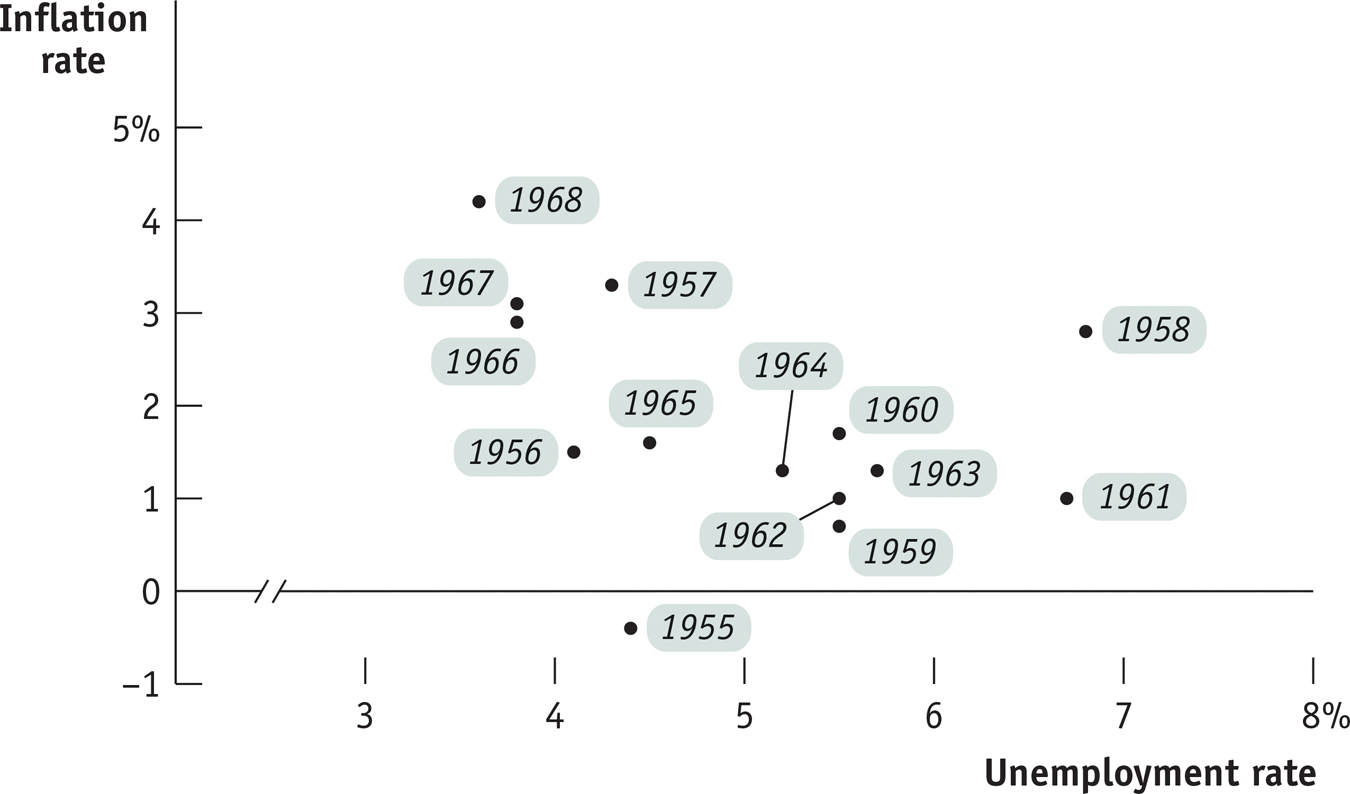
Unemployment and Inflation, 1955–1968 Each dot shows the average U.S. unemployment rate for one year and the percentage increase in the consumer price index over the subsequent year. Data like this lay behind the initial concept of the Phillips curve.Source: Bureau of Labor Statistics.
Looking at evidence like Figure 31-5, many economists concluded that there is a negative short-run relationship between the unemployment rate and the inflation rate, which is called the short-run Phillips curve, or SRPC. (We’ll explain the difference between the short-run and the long-run Phillips curve soon.) Figure 31-6 shows a hypothetical short-run Phillips curve.
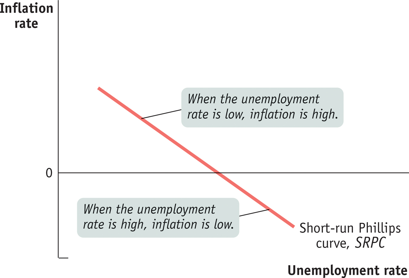
The Short-Run Phillips Curve The short-run Phillips curve, SRPC, slopes downward because the relationship between the unemployment rate and the inflation rate is negative.
The short-run Phillips curve is the negative short-run relationship between the unemployment rate and the inflation rate.
Early estimates of the short-run Phillips curve for the United States were very simple: they showed a negative relationship between the unemployment rate and the inflation rate, without taking account of any other variables. During the 1950s and 1960s, this simple approach seemed, for a while, to be adequate. And this simple relationship is clear in the data in Figure 31-5.
Even at the time, however, some economists argued that a more accurate short-run Phillips curve would include other factors. In Chapter 27 we discussed the effect of supply shocks, such as sudden changes in the price of oil, which shift the short-run aggregate supply curve. Such shocks also shift the short-run Phillips curve: surging oil prices were an important factor in the inflation of the 1970s and also played an important role in the acceleration of inflation in 2007–2008. In general, a negative supply shock shifts SRPC up as the inflation rate increases for every level of the unemployment rate, and a positive supply shock shifts it down as the inflation rate falls for every level of the unemployment rate. Both outcomes are shown in Figure 31-8.
FOR INQUIRING MINDS: The Aggregate Supply Curve and the Short-Run Phillips Curve
In earlier chapters we made extensive use of the AD–AS model, in which the short-run aggregate supply curve—a relationship between real GDP and the aggregate price level—plays a central role. Now we’ve introduced the concept of the short-run Phillips curve, a relationship between the unemployment rate and the rate of inflation. How do these two concepts fit together?
We can get a partial answer to this question by looking at panel (a) of Figure 31-7, which shows how changes in the aggregate price level and the output gap depend on changes in aggregate demand. Assume that in year 1 the aggregate demand curve is AD1, the long-run aggregate supply curve is LRAS, and the short-run aggregate supply curve is SRAS. The initial macroeconomic equilibrium is at E1, where the price level is 100 and real GDP is $10 trillion. Notice that at E1 real GDP is equal to potential output, so the output gap is zero.
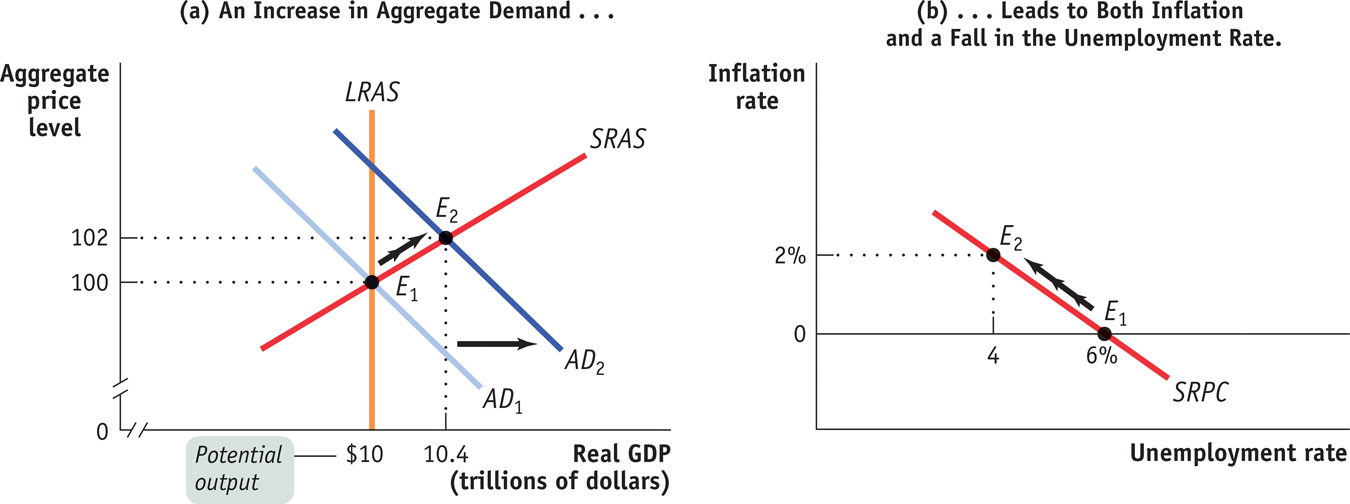
The AD–AS Model and the Short-Run Phillips Curve The short-run Phillips curve is closely related to the short-run aggregate supply curve. In panel (a), the economy is initially in equilibrium at E1, with the aggregate price level at 100 and aggregate output at $10 trillion, which we assume is potential output. Now consider two possibilities. If the aggregate demand curve remains at AD1, there is an output gap of zero and 0% inflation. If the aggregate demand curve shifts out to AD2, there is an output gap of 4%—reducing unemployment to 4%—and 2% inflation. Assuming that the natural rate of unemployment is 6%, the implications for unemployment and inflation are as follows, shown in panel (b): if aggregate demand does not increase, 6% unemployment and 0% inflation will result; if aggregate demand does increase, 4% unemployment and 2% inflation will result.
Now consider two possible paths for the economy over the next year. One is that aggregate demand remains unchanged and the economy stays at E1. The other is that aggregate demand shifts rightward to AD2 and the economy moves to E2.
At E2, real GDP is $10.4 trillion, $0.4 trillion more than potential output—a 4% output gap. Meanwhile, at E2 the aggregate price level is 102—a 2% increase. So panel (a) tells us that in this example, a zero output gap is associated with zero inflation and a 4% output gap is associated with 2% inflation.
Panel (b) shows what this implies for the relationship between unemployment and inflation. Assume that the natural rate of unemployment is 6% and that a rise of 1 percentage point in the output gap causes a fall of ½ percentage point in the unemployment rate per Okun’s law, described in the previous For Inquiring Minds. In that case, the two cases shown in panel (a)—aggregate demand either staying put or rising—correspond to the two points in panel (b). At E1, the unemployment rate is 6% and the inflation rate is 0%. At E2, the unemployment rate is 4%—because an output gap of 4% reduces the unemployment rate by 4% × 0.5 = 2% below its natural rate of 6%—and the inflation rate is 2%. So there is a negative relationship between unemployment and inflation.
So does the short-run aggregate supply curve say exactly the same thing as the short-run Phillips curve? Not quite. The short-run aggregate supply curve seems to imply a relationship between the change in the unemployment rate and the inflation rate, but the short-run Phillips curve shows a relationship between the level of the unemployment rate and the inflation rate. Reconciling these views completely would go beyond the scope of this book. The important point is that the short-run Phillips curve is a concept that is closely related, though not identical, to the short-run aggregate supply curve.
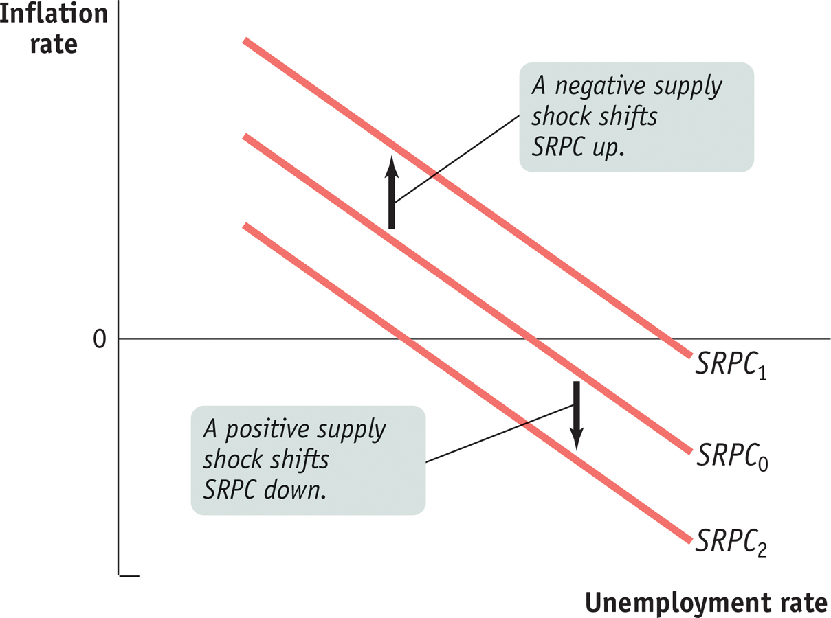
The Short-Run Phillips Curve and Supply Shocks A negative supply shock shifts the SRPC up, and a positive supply shock shifts the SRPC down.
But supply shocks are not the only factors that can change the inflation rate. In the early 1960s, Americans had little experience with inflation because inflation rates had been low for decades. But by the late 1960s, after inflation had been steadily increasing for a number of years, Americans had come to expect future inflation. In 1968, two economists—Milton Friedman of the University of Chicago and Edmund Phelps of Columbia University—independently set forth a crucial hypothesis: that expectations about future inflation directly affect the present inflation rate. Today most economists accept that the expected inflation rate—the rate of inflation that employers and workers expect in the near future—is the most important factor, other than the unemployment rate, affecting inflation.
Inflation Expectations and the Short-Run Phillips Curve
The expected rate of inflation is the rate of inflation that employers and workers expect in the near future. One of the crucial discoveries of modern macroeconomics is that changes in the expected rate of inflation affect the short-run trade-off between unemployment and inflation and shift the short-run Phillips curve.
Why do changes in expected inflation affect the short-run Phillips curve? Put yourself in the position of a worker and employer about to sign a contract setting the worker’s wages over the next year. For a number of reasons, the wage rate they agree to will be higher if everyone expects high inflation (including rising wages) than if everyone expects prices to be stable. The worker will want a wage rate that takes into account future declines in the purchasing power of earnings. He or she will also want a wage rate that won’t fall behind the wages of other workers. And the employer will be more willing to agree to a wage increase now if hiring workers later will be even more expensive. Also, rising prices will make paying a higher wage rate more affordable for the employer because the employer’s output will sell for more.
For these reasons, an increase in expected inflation shifts the short-run Phillips curve upward: the actual rate of inflation at any given unemployment rate is higher when the expected inflation rate is higher. In fact, macroeconomists believe that the relationship between changes in expected inflation and changes in actual inflation is one-to-one. That is, when the expected inflation rate increases, the actual inflation rate at any given unemployment rate will increase by the same amount. When the expected inflation rate falls, the actual inflation rate at any given level of unemployment will fall by the same amount.
Figure 31-9 shows how the expected rate of inflation affects the short-run Phillips curve. First, suppose that the expected rate of inflation is 0%. SRPC0 is the short-run Phillips curve when the public expects 0% inflation. According to SRPC0, the actual inflation rate will be 0% if the unemployment rate is 6%; it will be 2% if the unemployment rate is 4%.
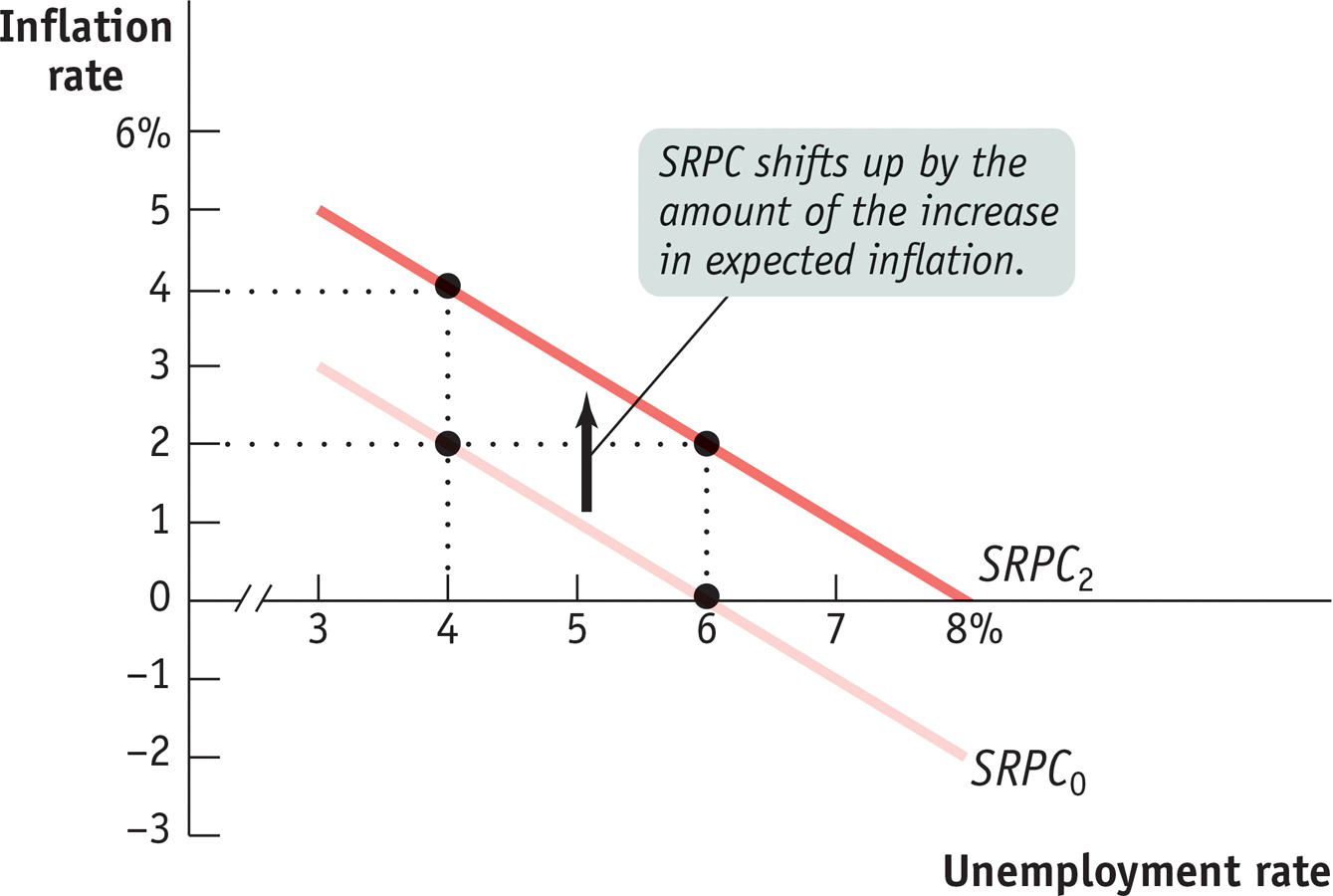
Expected Inflation and the Short-Run Phillips Curve An increase in expected inflation shifts the short-run Phillips curve up. SRPC0 is the initial short-run Phillips curve with an expected inflation rate of 0%; SRPC2 is the short-run Phillips curve with an expected inflation rate of 2%. Each additional percentage point of expected inflation raises the actual inflation rate at any given unemployment rate by 1 percentage point.
Alternatively, suppose the expected rate of inflation is 2%. In that case, employers and workers will build this expectation into wages and prices: at any given unemployment rate, the actual inflation rate will be 2 percentage points higher than it would be if people expected 0% inflation. SRPC2, which shows the Phillips curve when the expected inflation rate is 2%, is SRPC0 shifted upward by 2 percentage points at every level of unemployment. According to SRPC2, the actual inflation rate will be 2% if the unemployment rate is 6%; it will be 4% if the unemployment rate is 4%.
What determines the expected rate of inflation? In general, people base their expectations about inflation on experience. If the inflation rate has hovered around 0% in the last few years, people will expect it to be around 0% in the near future. But if the inflation rate has averaged around 5% lately, people will expect inflation to be around 5% in the near future.
Since expected inflation is an important part of the modern discussion about the short-run Phillips curve, you might wonder why it was not in the original formulation of the Phillips curve. The answer lies in history. Think back to what we said about the early 1960s: at that time, people were accustomed to low inflation rates and reasonably expected that future inflation rates would also be low. It was only after 1965 that persistent inflation became a fact of life. So only then did economists begin to argue that expected inflation should play an important role in price setting.
Sure enough, the seemingly clear relationship between inflation and unemployment fell apart after 1969. Figure 31-10 plots the track of U.S. unemployment and inflation rates from 1961 to 1990. As you can see, the track looks more like a tangled piece of yarn than like a smooth curve.
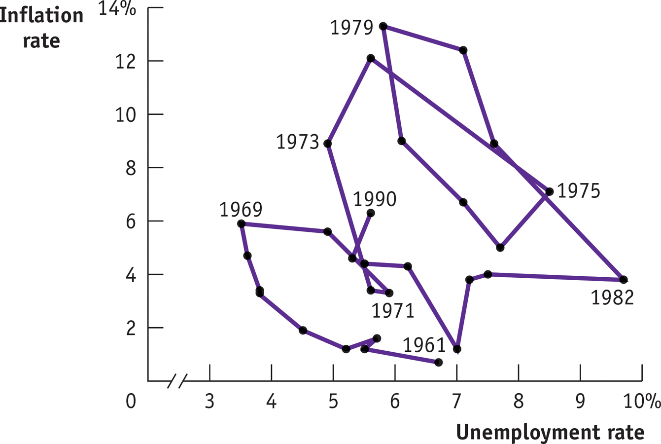
Unemployment and Inflation, 1961–1990 During the 1970s, the short-run Phillips curve relationship that seemed to hold during the 1950s and 1960s broke down as the U.S. economy experienced a combination of high unemployment and high inflation. Economists believe this was the result of both negative supply shocks and the cumulative effect of several years of higher than expected inflation. Inflation came down during the 1980s, and the 1990s were a time of both low unemployment and low inflation.Source: Bureau of Labor Statistics.
Through much of the 1970s and early 1980s, the economy suffered from a combination of above-average unemployment rates coupled with inflation rates unprecedented in modern American history. This condition came to be known as stagflation—for stagnation combined with high inflation. In the late 1990s, by contrast, the economy was experiencing a blissful combination of low unemployment and low inflation. What explains these developments?
Part of the answer can be attributed to a series of negative supply shocks that the U.S. economy suffered during the 1970s. The price of oil, in particular, soared as wars and revolutions in the Middle East led to a reduction in oil supplies and as oil-exporting countries deliberately curbed production to drive up prices. Compounding the oil price shocks, there was also a slowdown in labor productivity growth. Both of these factors shifted the short-run Phillips curve upward. During the 1990s, by contrast, supply shocks were positive. Prices of oil and other raw materials were generally falling, and productivity growth accelerated. As a result, the short-run Phillips curve shifted downward.
Equally important, however, was the role of expected inflation. As mentioned earlier in the chapter, inflation accelerated during the 1960s. During the 1970s, the public came to expect high inflation, and this also shifted the short-run Phillips curve up. It took a sustained and costly effort during the 1980s to get inflation back down. The result, however, was that expected inflation was very low by the late 1990s, allowing actual inflation to be low even with low rates of unemployment.
!worldview! ECONOMICS in Action: The Phillips Curve in the Great Recession
The Phillips Curve in the Great Recession
We have returned many times in the course of this book to the great global economic crisis that struck in 2008. This crisis caused a drastic rise in unemployment in many countries, especially in some (but not all) European nations, and unemployment remained high even years later. According to the logic of the Phillips curve, this surge in unemployment should have led to falling inflation, with the biggest declines in the worst-hit countries. And that is exactly what happened.
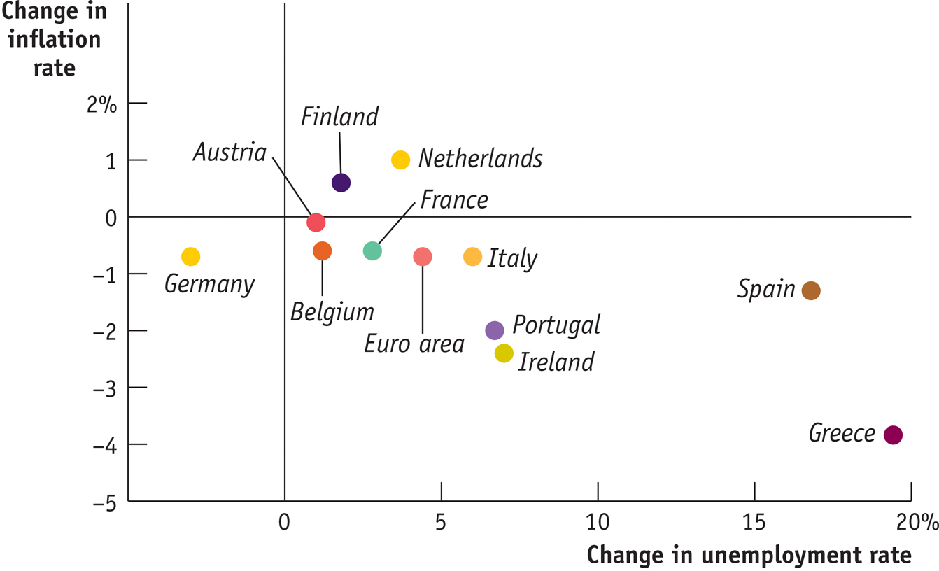
Rising Unemployment, Falling Inflation in Europe, 2007–2013Source: IMF World Economic Outlook.
Figure 31-11 shows how unemployment rates and inflation rates in a number of European economies changed between 2007, the eve of the Great Recession, and 2013. Unemployment rose in every country except Germany, soaring in Ireland and the troubled economies of southern Europe. Inflation fell in 9 out of 12 countries, falling much more than the average in those same troubled economies. The relationship between unemployment and inflation isn’t exact—relationships in economics rarely are. But the data are consistent with the notion of a short-run trade-off between unemployment and inflation. Incidentally, researchers at the Federal Reserve have found a similar relationship between unemployment and inflation among major U.S. metropolitan areas, some of which were hit much harder by the housing bust than others.
Quick Review
Okun’s law describes the relationship between the output gap and cyclical unemployment.
The short-run Phillips curve illustrates the negative relationship between unemployment and inflation.
A negative supply shock shifts the short-run Phillips curve upward, but a positive supply shock shifts it downward.
An increase in the expected rate of inflation pushes the short-run Phillips curve upward: each additional percentage point of expected inflation pushes the actual inflation rate at any given unemployment rate up by 1 percentage point.
In the 1970s, a series of negative supply shocks and a slowdown in labor productivity growth led to stagflation and an upward shift in the short-run Phillips curve.
31-2
Question
16.3
Explain how the short-run Phillips curve illustrates the negative relationship between cyclical unemployment and the actual inflation rate for a given level of the expected inflation rate.
Question
16.4
Which way does the short-run Phillips curve move in response to a fall in commodities prices? To a surge in commodities prices? Explain.
Solutions appear at back of book.