5.2 Interpreting the Price Elasticity of Demand
In a true emergency, a patient is unlikely to question the price of the ambulance ride to the hospital. But even in a non-
To answer these questions, we need to look more deeply at the price elasticity of demand.
How Elastic Is Elastic?
As a first step toward classifying price elasticities of demand, let’s look at the extreme cases.
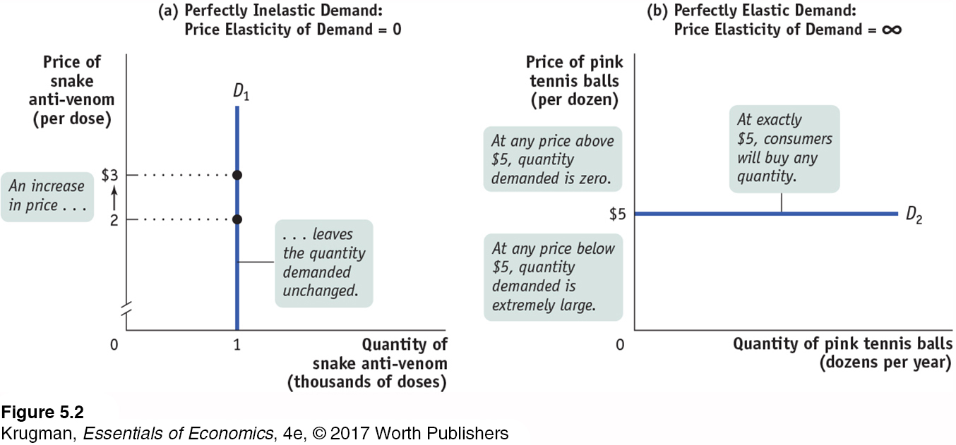
Demand is perfectly inelastic when the quantity demanded does not respond at all to changes in the price. When demand is perfectly inelastic, the demand curve is a vertical line.
First, consider the demand for a good when people pay no attention to the price—
143
The opposite extreme occurs when even a tiny rise in the price will cause the quantity demanded to drop to zero or even a tiny fall in the price will cause the quantity demanded to get extremely large.
Demand is perfectly elastic when any price increase will cause the quantity demanded to drop to zero. When demand is perfectly elastic, the demand curve is a horizontal line.
Panel (b) of Figure 5-2 shows the case of pink tennis balls; we suppose that tennis players really don’t care what color their balls are and that other colors, such as neon green and vivid yellow, are available at $5 per dozen balls. In this case, consumers will buy no pink balls if they cost more than $5 per dozen but will buy only pink balls if they cost less than $5. The demand curve will therefore be a horizontal line at a price of $5 per dozen balls. As you move back and forth along this line, there is a change in the quantity demanded but no change in the price. Roughly speaking, when you divide a number by zero, you get infinity, denoted by the symbol ∞. So a horizontal demand curve implies an infinite price elasticity of demand. When the price elasticity of demand is infinite, economists say that demand is perfectly elastic.
Demand is elastic if the price elasticity of demand is greater than 1, inelastic if the price elasticity of demand is less than 1, and unit-
The price elasticity of demand for the vast majority of goods is somewhere between these two extreme cases. Economists use one main criterion for classifying these intermediate cases: they ask whether the price elasticity of demand is greater or less than 1. When the price elasticity of demand is greater than 1, economists say that demand is elastic. When the price elasticity of demand is less than 1, they say that demand is inelastic. The borderline case is unit-
To see why a price elasticity of demand equal to 1 is a useful dividing line, let’s consider a hypothetical example: a toll bridge operated by the state highway department. Other things equal, the number of drivers who use the bridge depends on the toll, the price the highway department charges for crossing the bridge: the higher the toll, the fewer the drivers who use the bridge.
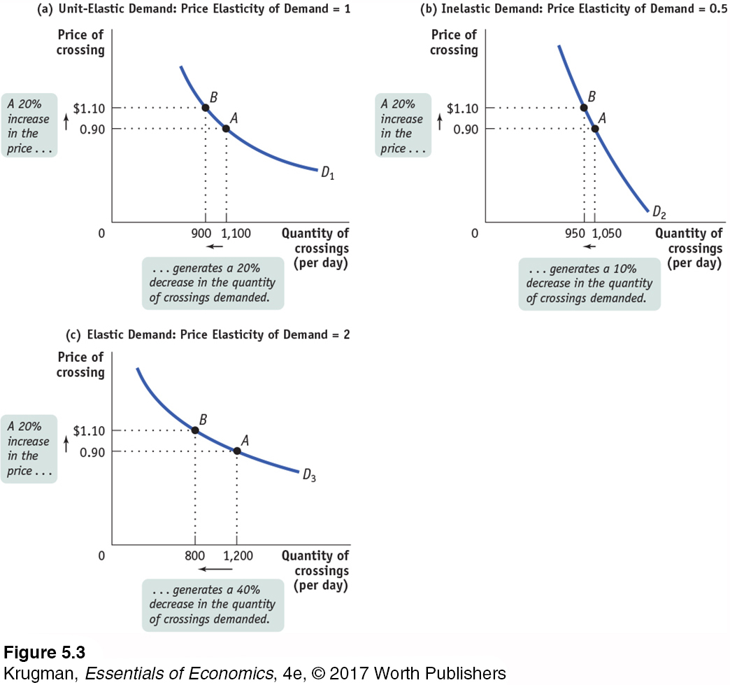
Figure 5-3 shows three hypothetical demand curves—
Panel (a) shows what happens when the toll is raised from $0.90 to $1.10 and the demand curve is unit-
Panel (b) shows a case of inelastic demand when the toll is raised from $0.90 to $1.10. The same 20% price rise reduces the quantity demanded from 1,050 to 950. That’s only a 10% decline, so in this case the price elasticity of demand is 10%/20% = 0.5.
Panel (c) shows a case of elastic demand when the toll is raised from $0.90 to $1.10. The 20% price increase causes the quantity demanded to fall from 1,200 to 800—
The total revenue is the total value of sales of a good or service. It is equal to the price multiplied by the quantity sold.
Why does it matter whether demand is unit-
(5-
144
Total revenue has a useful graphical representation that can help us understand why knowing the price elasticity of demand is crucial when we ask whether a price rise will increase or reduce total revenue. Panel (a) of Figure 5-4 shows the same demand curve as panel (a) of Figure 5-3. We see that 1,100 drivers will use the bridge if the toll is $0.90. So the total revenue at a price of $0.90 is $0.90 × 1,100 = $990. This value is equal to the area of the green rectangle, which is drawn with the bottom left corner at the point (0, 0) and the top right corner at (1,100, 0.90). In general, the total revenue at any given price is equal to the area of a rectangle whose height is the price and whose width is the quantity demanded at that price.
To get an idea of why total revenue is important, consider the following scenario. Suppose that the toll on the bridge is currently $0.90 but that the highway department must raise extra money for road repairs. One way to do this is to raise the toll on the bridge. But this plan might backfire, since a higher toll will reduce the number of drivers who use the bridge. And if traffic on the bridge dropped a lot, a higher toll would actually reduce total revenue instead of increasing it. So it’s important for the highway department to know how drivers will respond to a toll increase.
145
We can see graphically how the toll increase affects total bridge revenue by examining panel (b) of Figure 5-4. At a toll of $0.90, total revenue is given by the sum of the areas A and B. After the toll is raised to $1.10, total revenue is given by the sum of areas B and C. So when the toll is raised, revenue represented by area A is lost but revenue represented by area C is gained.
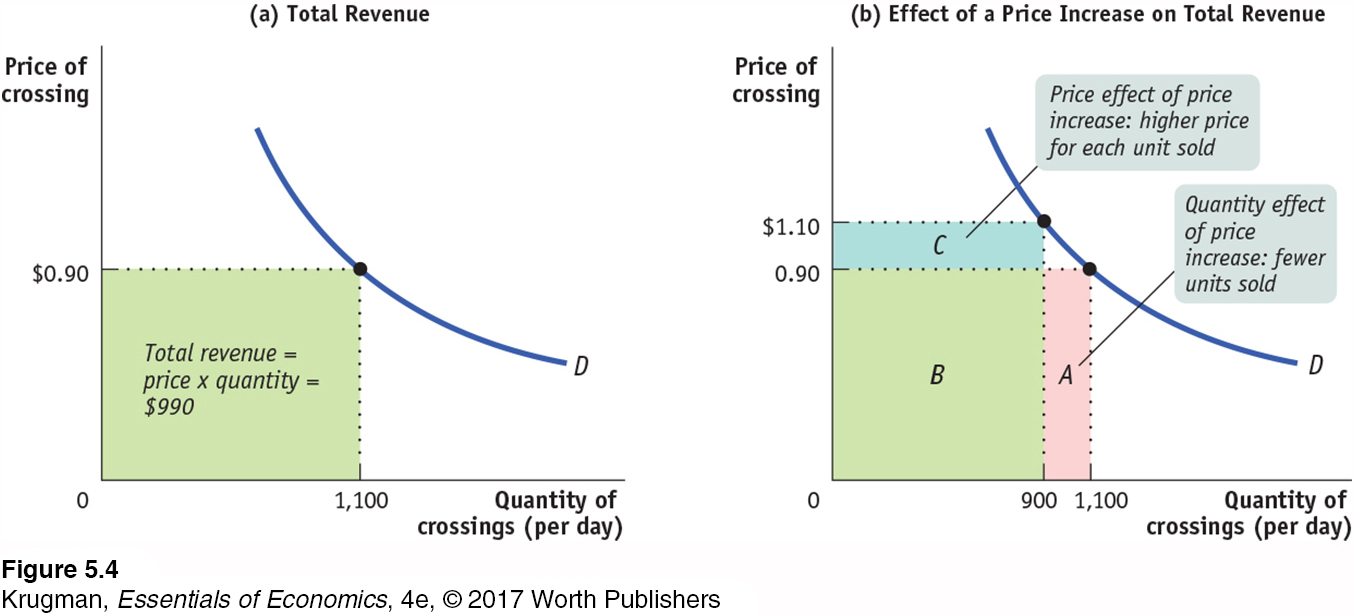
These two areas have important interpretations. Area C represents the revenue gain that comes from the additional $0.20 paid by drivers who continue to use the bridge. That is, the 900 who continue to use the bridge contribute an additional $0.20 × 900 = $180 per day to total revenue, represented by area C. But 200 drivers who would have used the bridge at a price of $0.90 no longer do so, generating a loss to total revenue of $0.90 × 200 = $180 per day, represented by area A. (In this particular example, because demand is unit-

Except in the rare case of a good with perfectly elastic or perfectly inelastic demand, when a seller raises the price of a good, two countervailing effects are present:
A price effect: After a price increase, each unit sold sells at a higher price, which tends to raise revenue.
A quantity effect: After a price increase, fewer units are sold, which tends to lower revenue.
146
But then, you may ask, what is the ultimate net effect on total revenue: does it go up or down? The answer is that, in general, the effect on total revenue can go either way—
The price elasticity of demand tells us what happens to total revenue when price changes: its size determines which effect—
If demand for a good is unit-
elastic (the price elasticity of demand is 1), an increase in price does not change total revenue. In this case, the quantity effect and the price effect exactly offset each other. If demand for a good is inelastic (the price elasticity of demand is less than 1), a higher price increases total revenue. In this case, the quantity effect is weaker than the price effect.
If demand for a good is elastic (the price elasticity of demand is greater than 1), an increase in price reduces total revenue. In this case, the quantity effect is stronger than the price effect.
Table 5-2 shows how the effect of a price increase on total revenue depends on the price elasticity of demand, using the same data as in Figure 5-3. An increase in the price from $0.90 to $1.10 leaves total revenue unchanged at $990 when demand is unit-
The price elasticity of demand also predicts the effect of a fall in price on total revenue. When the price falls, the same two countervailing effects are present, but they work in the opposite directions as compared to the case of a price rise. There is the price effect of a lower price per unit sold, which tends to lower revenue. This is countered by the quantity effect of more units sold, which tends to raise revenue. Which effect dominates depends on the price elasticity. Here is a quick summary:
When demand is unit-
elastic, the two effects exactly balance; so a fall in price has no effect on total revenue. When demand is inelastic, the quantity effect is dominated by the price effect; so a fall in price reduces total revenue.
147
When demand is elastic, the quantity effect dominates the price effect; so a fall in price increases total revenue.
| Price of toll = $0.90 | Price of toll = $1.10 | |
|
Unit- (price elasticity of demand = 1) |
||
| Quantity demanded | 1,100 | 900 |
| Total revenue | $990 | $990 |
|
Inelastic demand (price elasticity of demand = 0.5) |
||
| Quantity demanded | 1,050 | 950 |
| Total revenue | $945 | $1,045 |
|
Elastic demand (price elasticity of demand = 2) |
||
| Quantity demanded | 1,200 | 800 |
| Total revenue | $1,080 | $880 |
Price Elasticity Along the Demand Curve
Suppose an economist says that “the price elasticity of demand for coffee is 0.25.” What he or she means is that at the current price the elasticity is 0.25. In the previous discussion of the toll bridge, what we were really describing was the elasticity at the price of $0.90. Why this qualification? Because for the vast majority of demand curves, the price elasticity of demand at one point along the curve is different from the price elasticity of demand at other points along the same curve.
To see this, consider the table in Figure 5-5, which shows a hypothetical demand schedule. It also shows in the last column the total revenue generated at each price and quantity combination in the demand schedule. The upper panel of the graph in Figure 5-5 shows the corresponding demand curve. The lower panel illustrates the same data on total revenue: the height of a bar at each quantity demanded—
148
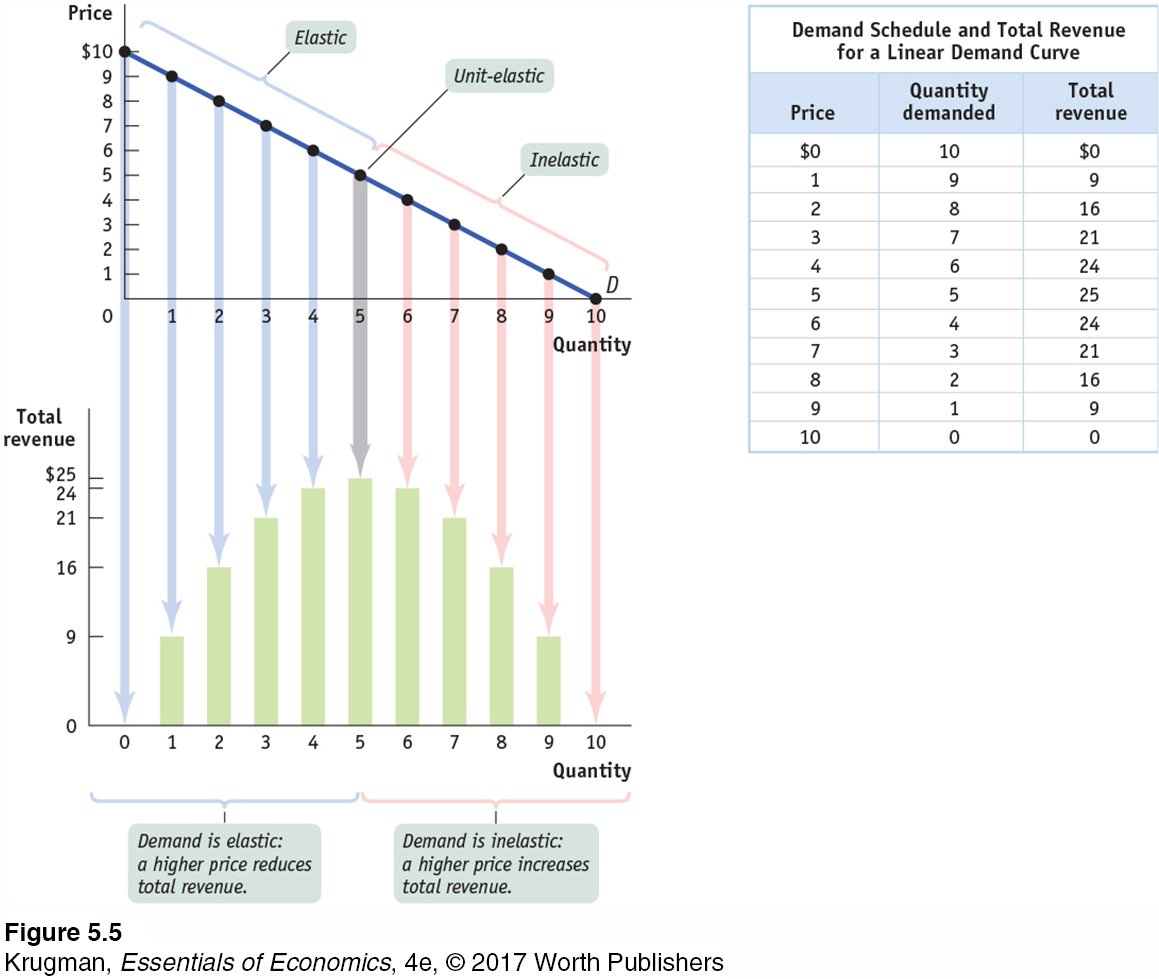
In Figure 5-5, you can see that when the price is low, raising the price increases total revenue: starting at a price of $1, raising the price to $2 increases total revenue from $9 to $16. This means that when the price is low, demand is inelastic. Moreover, you can see that demand is inelastic on the entire section of the demand curve from a price of $0 to a price of $5.
When the price is high, however, raising it further reduces total revenue: starting at a price of $8, raising the price to $9 reduces total revenue, from $16 to $9. This means that when the price is high, demand is elastic. Furthermore, you can see that demand is elastic over the section of the demand curve from a price of $5 to $10.
For the vast majority of goods, the price elasticity of demand changes along the demand curve. So whenever you measure a good’s elasticity, you are really measuring it at a particular point or section of the good’s demand curve.
What Factors Determine the Price Elasticity of Demand?
Investors in private ambulance companies believe that the price elasticity of demand for an ambulance ride is low for two important reasons. First, in many if not most cases, an ambulance ride is a medical necessity. Second, in an emergency there really is no substitute for the standard of care that an ambulance provides. And even among ambulances there are typically no substitutes because in any given geographical area there is usually only one ambulance provider. (The exceptions are very densely populated areas, but even in those locations an ambulance dispatcher is unlikely to give you a choice of ambulance providers with an accompanying price list.)
In general there are four main factors that determine elasticity: whether a good is a necessity or luxury, the availability of close substitutes, the share of income a consumer spends on the good, and how much time has elapsed since a change in price. We’ll briefly examine each of these factors.
Whether the Good Is a Necessity or a Luxury As our opening story illustrates, the price elasticity of demand tends to be low if a good is something you must have, like a life-
The Availability of Close Substitutes As we just noted, the price elasticity of demand tends to be low if there are no close substitutes or if they are very difficult to obtain. In contrast, the price elasticity of demand tends to be high if there are other readily available goods that consumers regard as similar and would be willing to consume instead. For example, most consumers believe that there are fairly close substitutes to their favorite brand of breakfast cereal. As a result, if the maker of a particular brand of breakfast cereal raised the price significantly, that maker is likely to lose much—
Share of Income Spent on the Good Consider a good that some people consume frequently, such as gasoline—
149
Time Elapsed Since Price Change In general, the price elasticity of demand tends to increase as consumers have more time to adjust. This means that the long-
A good illustration is the changes in Americans’ behavior over the past decade in response to higher gasoline prices. In 1998, a gallon of gasoline was only about $1. Over the years, however, gasoline prices steadily rose, so by early 2013 a gallon of gas cost from $3.50 to $4.00 in much of the United States. Over time, however, people changed their habits and choices in ways that enabled them to gradually reduce their gasoline consumption. In a recent survey, 53% of responders said they had made major life changes in order to cope with higher gas prices—
ECONOMICS in Action
Responding to Your Tuition Bill
![]() | interactive activity
| interactive activity
College costs more than ever—
A 1988 study found that a 3% increase in tuition led to an approximately 2% fall in the number of students enrolled at four-

A 1999 study confirmed this pattern. In comparison to four-
150
In response to decreased state funding, many public colleges and universities have been experimenting with changes to their tuition schedule in order to increase revenue. A 2012 study found that in-
Not surprisingly, many public colleges and universities have found that raising the tuition for enrollments of out-
Quick Review
Demand is perfectly inelastic if it is completely unresponsive to price. It is perfectly elastic if it is infinitely responsive to price.
Demand is elastic if the price elasticity of demand is greater than 1. It is inelastic if the price elasticity of demand is less than 1. It is unit-
elastic if the price elasticity of demand is exactly 1. When demand is elastic, the quantity effect of a price increase dominates the price effect and total revenue falls. When demand is inelastic, the price effect of a price increase dominates the quantity effect and total revenue rises.
Because the price elasticity of demand can change along the demand curve, economists refer to a particular point on the demand curve when speaking of “the” price elasticity of demand.
Ready availability of close substitutes makes demand for a good more elastic, as does a longer length of time elapsed since the price change. Demand for a necessity is less elastic, and demand for a luxury good is more elastic. Demand tends to be inelastic for goods that absorb a small share of a consumer’s income and elastic for goods that absorb a large share of income.
Check Your Understanding 5-
Question 5.4
1. For each case, choose the condition that characterizes demand: elastic demand, inelastic demand, or unit-
Total revenue decreases when price increases.
Elastic demand. Consumers are highly responsive to changes in price. For a rise in price, the quantity effect (which tends to reduce total revenue) outweighs the price effect (which tends to increase total revenue). Overall, this leads to a fall in total revenue.
The additional revenue generated by an increase in quantity sold is exactly offset by revenue lost from the fall in price received per unit.
Unit-
elastic demand. Here the revenue lost to the fall in price is exactly equal to the revenue gained from higher sales. The quantity effect exactly offsets the price effect. Total revenue falls when output increases.
Inelastic demand. Consumers are relatively unresponsive to changes in price. For consumers to purchase a given percent increase in output, the price must fall by an even greater percent. The price effect of a fall in price (which tends to reduce total revenue) outweighs the quantity effect (which tends to increase total revenue). As a result, total revenue decreases.
Producers in an industry find they can increase their total revenues by coordinating a reduction in industry output.
Inelastic demand. Consumers are relatively unresponsive to price, so the percent fall in output is smaller than the percent rise in price. The price effect of a rise in price (which tends to increase total revenue) outweighs the quantity effect (which tends to reduce total revenue). As a result, total revenue increases.
Question 5.5
2. For the following goods, what is the elasticity of demand? Explain. What is the shape of the demand curve?
Demand for a blood transfusion by an accident victim
The demand of an accident victim for a blood transfusion is very likely to be perfectly inelastic because there is no substitute and it is necessary for survival. The demand curve will be vertical, at a quantity equal to the needed transfusion quantity.
Demand by students for green erasers
Students’ demand for green erasers is likely to be perfectly elastic because there are easily available substitutes: nongreen erasers. The demand curve will be horizontal, at a price equal to that of nongreen erasers.
Solutions appear at back of book.