Worked Problem: A Shocking Analysis
During the financial crisis in autumn 2008, the financial system delivered a sobering shock to the economy when the stock market lost about half of its value. Soon afterward, consumer spending came to a screeching halt. Within six months of the crash, GDP fell by 2.5% and the price level fell by 2.8%. Show how an analysis of aggregate demand and aggregate supply could have predicted this short-run effect on aggregate output and the aggregate price level. Assuming no government intervention, what would you have predicted in the long run?
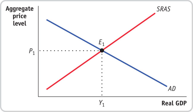
Draw and label the aggregate demand curve and the short-run aggregate supply curve. Find and label the initial equilibrium point, the initial price level, and the initial output level.
Read the section “Short-Run Macroeconomic Equilibrium” beginning on page 428. Study Figure 14-9. Label the horizontal axis “Real GDP,” the vertical axis “Aggregate price level,” and the initial equilibrium point E1. The initial price level and output levels should be labeled P1 and Y1, respectively.
The aggregate demand curve and the short-run aggregate supply curve are shown in the diagram below. The initial equilibrium point is labeled E1, the initial price level is labeled P1, and the initial output level is labeled Y1. 
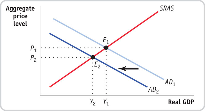
Using your figure from Step 1, analyze the short-run effect of the stock market fall on aggregate demand and aggregate supply by drawing a new curve representing aggregate demand after the stock market fall.
Read the section “Shifts of the Aggregate Demand Curve” beginning on page 414. A fall in the stock market represents a fall in the real value of household assets. Then read the section, “Shifts of Aggregate Demand: Short-Run Effects” beginning on page 429. Study panel (a) of Figure 14-10. Label the initial aggregate demand curve “AD1,” and the aggregate demand curve after the stock market fall “AD2.”
A decrease in household wealth will reduce consumer spending. Beginning at the equilibrium point, E1 in the accompanying diagram, the aggregate demand curve will shift from AD1 to AD2. The economy will be in short-run macroeconomic equilibrium at point E2. The aggregate price level will be lower than at P1, and aggregate output will be lower than output at the original equilibrium point.
441
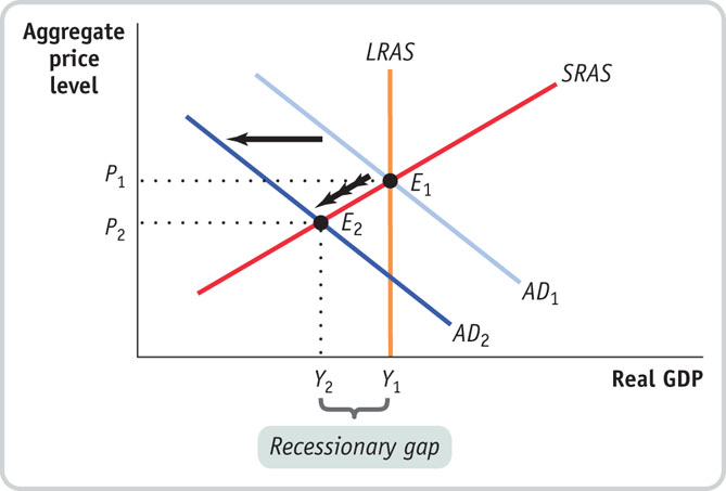
Draw the long-run aggregate supply curve through the initial equilibrium point E{{sub}}1{{/sub}}, and label the recessionary gap.
Read the first part of the section “Long-Run Macroeconomic Equilibrium” beginning on page 432. Study Figures 14-12 and 14-13 on page 433.
The long-run aggregate supply curve is drawn in the diagram below. The economy now faces a recessionary gap between Y1 and Y2.
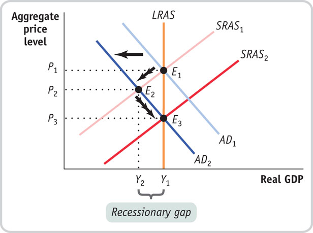
What would you predict in the long run?
Read the section, “Long-Run Macroeconomic Equilibrium” beginning on page 432. Study Figure 14-13 on page 433.
As wage contracts are renegotiated, nominal wages will fall and the short-run aggregate supply curve will shift gradually to the right over time until it reaches SRAS2 and intersects AD2 at point E3. At E3, the economy is back at its potential output but at a much lower aggregate price level.
442