Defining and Measuring Elasticity
In order for Flunomics, a hypothetical flu vaccine distributor, to know whether it could raise its revenue by significantly raising the price of its flu vaccine during the 2004 flu vaccine panic, it would have to know the price elasticity of demand for flu vaccinations.
Calculating the Price Elasticity of Demand
Figure 5-1 shows a hypothetical demand curve for flu vaccinations. At a price of $20 per vaccination, consumers would demand 10 million vaccinations per year (point A); at a price of $21, the quantity demanded would fall to 9.9 million vaccinations per year (point B).
Figure 5-1, then, tells us the change in the quantity demanded for a particular change in the price. But how can we turn this into a measure of price responsiveness? The answer is to calculate the price elasticity of demand.
The price elasticity of demand is the ratio of the percent change in the quantity demanded to the percent change in the price as we move along the demand curve (dropping the minus sign).
The price elasticity of demand is the ratio of the percent change in quantity demanded to the percent change in price as we move along the demand curve. As we’ll see later in this chapter, the reason economists use percent changes is to obtain a measure that doesn’t depend on the units in which a good is measured (say, a child-size dose versus an adult-size dose of vaccine). But before we get to that, let’s look at how elasticity is calculated.
To calculate the price elasticity of demand, we first calculate the percent change in the quantity demanded and the corresponding percent change in the price as we move along the demand curve. These are defined as follows:

and

In Figure 5-1, we see that when the price rises from $20 to $21, the quantity demanded falls from 10 million to 9.9 million vaccinations, yielding a change in the quantity demanded of 0.1 million vaccinations. So the percent change in the quantity demanded is


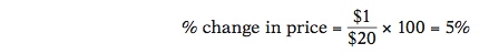
The initial price is $20 and the change in the price is $1, so the percent change in price is
To calculate the price elasticity of demand, we find the ratio of the percent change in the quantity demanded to the percent change in the price:

In Figure 5-1, the price elasticity of demand is therefore

The law of demand says that demand curves are downward sloping, so price and quantity demanded always move in opposite directions. In other words, a positive percent change in price (a rise in price) leads to a negative percent change in the quantity demanded; a negative percent change in price (a fall in price) leads to a positive percent change in the quantity demanded. This means that the price elasticity of demand is, in strictly mathematical terms, a negative number. However, it is inconvenient to repeatedly write a minus sign. So when economists talk about the price elasticity of demand, they usually drop the minus sign and report the absolute value of the price elasticity of demand. In this case, for example, economists would usually say “the price elasticity of demand is 0.2,” taking it for granted that you understand they mean minus 0.2. We follow this convention here.
145
The larger the price elasticity of demand, the more responsive the quantity demanded is to the price. When the price elasticity of demand is large—when consumers change their quantity demanded by a large percentage compared with the percent change in the price—economists say that demand is highly elastic.
As we’ll see shortly, a price elasticity of 0.2 indicates a small response of quantity demanded to price. That is, the quantity demanded will fall by a relatively small amount when price rises. This is what economists call inelastic demand. And inelastic demand was exactly what Flunomics needed for its strategy to increase revenue by raising the price of its flu vaccines.
An Alternative Way to Calculate Elasticities: The Midpoint Method
Price elasticity of demand compares the percent change in quantity demanded with the percent change in price. When we look at some other elasticities, which we will do shortly, we’ll learn why it is important to focus on percent changes. But at this point we need to discuss a technical issue that arises when you calculate percent changes in variables.
The best way to understand the issue is with a real example. Suppose you were trying to estimate the price elasticity of demand for gasoline by comparing gasoline prices and consumption in different countries. Because of high taxes, gasoline usually costs about three times as much per gallon in Europe as it does in the United States. So what is the percent difference between American and European gas prices?
146
Well, it depends on which way you measure it. Because the price of gasoline in Europe is approximately three times higher than in the United States, it is 200 percent higher. Because the price of gasoline in the United States is one-third as high as in Europe, it is 66.7 percent lower.
This is a nuisance: we’d like to have a percent measure of the difference in prices that doesn’t depend on which way you measure it. To avoid computing different elasticities for rising and falling prices we use the midpoint method.
The midpoint method replaces the usual definition of the percent change in a variable, X, with a slightly different definition:
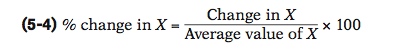
where the average value of X is defined as

The midpoint method is a technique for calculating the percent change. In this approach, we calculate changes in a variable compared with the average, or midpoint, of the starting and final values.
When calculating the price elasticity of demand using the midpoint method, both the percent change in the price and the percent change in the quantity demanded are found using this method. To see how this method works, suppose you have the following data for some good:
| Price | Quantity demanded | |
|---|---|---|
| Situation A | $0.90 | 1,100 |
| Situation B | $1.10 | 900 |
To calculate the percent change in quantity going from situation A to situation B, we compare the change in the quantity demanded—a fall of 200 units—with the average of the quantity demanded in the two situations. So we calculate

In the same way, we calculate

So in this case we would calculate the price elasticity of demand to be

again dropping the minus sign.
The important point is that we would get the same result, a price elasticity of demand of 1, whether we go up the demand curve from situation A to situation B or down from situation B to situation A.
To arrive at a more general formula for price elasticity of demand, suppose that we have data for two points on a demand curve. At point 1 the quantity demanded and price are (Q1, P1); at point 2 they are (Q2, P2). Then the formula for calculating the price elasticity of demand is:
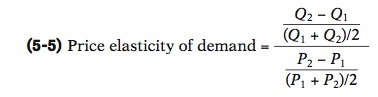
As before, when finding a price elasticity of demand calculated by the midpoint method, we drop the minus sign and use the absolute value.
147
Estimating Elasticities
You might think it’s easy to estimate price elasticities of demand from real-world data: just compare percent changes in prices with percent changes in quantities demanded. Unfortunately, it’s rarely that simple because changes in price aren’t the only thing affecting changes in the quantity demanded: other factors—such as changes in income, changes in tastes, and changes in the prices of other goods—shift the demand curve, thereby changing the quantity demanded at any given price. To estimate price elasticities of demand, economists must use careful statistical analysis to separate the influence of these different factors, holding other things equal.
The most comprehensive effort to estimate price elasticities of demand was a mammoth study by the economists Hendrik S. Houthakker and Lester D. Taylor. Some of their results are summarized in Table 5-1. These estimates show a wide range of price elasticities. There are some goods, like eggs, for which demand hardly responds at all to changes in the price. There are other goods, most notably foreign travel, for which the quantity demanded is very sensitive to the price.
| Good | Price elasticity of demand |
|---|---|
| Inelastic demand | |
| Eggs | 0.1 |
| Beef | 0.4 |
| Stationery | 0.5 |
| Gasoline | 0.5 |
| Elastic demand | |
| Housing | 1.2 |
| Restaurant meals | 2.3 |
| Airline travel | 2.4 |
| Foreign travel | 4.1 |
| Source note on copyright page. | |
Notice that Table 5-1 is divided into two parts: inelastic and elastic demand. We’ll explain in the next section the significance of that division.
Quick Review
- The price elasticity of demand is equal to the percent change in the quantity demanded divided by the percent change in the price as you move along the demand curve, and dropping any minus sign.
- In practice, percent changes are best measured using the midpoint method, in which the percent change in each variable is calculated using the average of starting and final values.
Check Your Understanding 5-1
Question
TvY8CZwM9RBeS3lG2n4RU84oj43CbQWw3oQOit/IgbIH541WCfUo/IdKfFc7Y0lGz7sFoGXycrIciFuRgQzXgFmlwY8J3Qc3ckA1WBGMShLyfJFVYXMgOIkP1qG2gxCu1O6nJbTSl42b7YTvl2uRdIAmmP6yHQuyPHgnx15E6E6NWexS48v70yloISiVSTaTLGivm7yZmiEyi9rO9DC+gWO5un/j+51REBIaDm/r8B6w727l1yU70SO9sSU3nKFpe0dYJcnIPebHDlGanpuOZee3Di/99dDYBsHr8jG8F9izyUFbIgl+swWbobDIRmAje+VqCh3DJ9c=The price elasticity of demand using the midpoint method is 67% / 40% = 1.7Question
YxKqqxCx3fztV8hbUAzaClpx5JvJ6VF9IJYdIoxEnk1d1MJJuvbO88i+VhTqr22g31Ukl3canlo6VRI24gnOqpr9d03aIUPrpZDoFGHeQXqqdoimbnYdBLhtL+iQj3badGMXLG+dtg5Tzd+6ya44zH7XGv8p89CuPZf/AMswOJHwkwR5NsfLGMYAPHxTAulb2GSZ2p2GAM+QUtf/B3zdZ4G77+FB4J4eRa6S/1eXbAREAinFpAEMKHPs71RgbKcz1pzwk6zrVt6GiBDjWsHY0USi4EgJiQlGEhcCANPB4uF7ji94aeEBOQHz1zo0XDr40XEsEpjZQeSOP0WMn+VjVhpnl/gNrc0CvF/4ErbDpAcGiWbHFRjvv/GsayTARldctsuTlCFaOli8/o1ntJ0VQi5VHs3zFUGP0ggSTbv9KXzaYsphD1XdpalM0ce44vGyTUtW94fOnwJQCZuauX9KjW0CIeilZ7cesxTI15VG7Ey4S6DIbcUXwMBi4rS9Rr86ApUPpASuMFkF7+Rj23zk4w==Since the price elasticity of demand is 1 at the current consumption level, and the percentage change in quantity demanded amounts to ((5,000 - 4,000)/((4,000 + 5,000)/2)) * 100 = 22%, then it will take a 22% reduction in the price of movie tickets to generate a 22% increase in quantity demanded.Question
YqgXESAmnwO/43Wh4JtE7HenFqd6Wphf1zVg8/wwzNs3RGEK5n14ZnSht25Lq1eAurCQyfEyV7YO7a8XfbnXNJN6h0oy50HZoK5Ms3906pfgR6N4MM7ehwV+penyb6AsN20kRj1YQk+PfPMXWmPm64zdPw/U4/6c4KzMCADTemtwxhqunnY5PGRpzV5s27lV0UkPwHRdAVIG2hmglmwe5Lcn4VBCnMF8YH7KjMI9PS8OZgG0EBO+E5HG1jNVt/ZlSZkPSjrSbMe0DR2sXxeNynLuyWuzfRLinU9KMURbxH1qS5eFNmMqXPdRKEh7WfYCg1jKFXGS3fOMy2TnL8zR0XkoBZ2mV8mmiYV3QmugLO7R4ChaDRzZX4zHuKFDhU9JsBiKY/YoTkzQvmWho6uwd4xGupLgKPYq1mUfRSVxeY9AcQBpBkX+aV0BQzscRw71SNWshralHRWBOADqH+5DKX8s29B8x6MoBXmowAPZ6eNwxIHcBqiEAubE4/Gej2KhIqa/sWDezKLVdl/xBJ3fGpqWQmrvF36X9JdgZMmou81Nnk6sNkSRCE3u2qw=Since price rises, we know that quantity demanded must fall. Given the current price of $0.50, a $0.05 increase in price represents a 10% change, using the method in Equation 5-2. So the price elasticity of demand is change in quantity demanded / 10% = 1.2 so that the percent change in quantity demanded is 12%. A 12% decrease in quantity demanded represents 100,000 × 0.12, or 12,000 sandwiches.
Solutions appear at back of book.