Worked Problem: Reducing Greenhouse Gases
In July 2009, the House of Representatives passed the American Clean Energy and Security Act. Part of the bill provides for a cap and trade program for greenhouse gases. In a cap and trade program, the government sets a legal limit (a cap) on the amount of pollutant that can be emitted. In order to identify the cap, the government should apply the principle of marginal analysis, setting the marginal social cost of pollution equal to the marginal social benefit of pollution. But how can pollution have a marginal social benefit?
As we saw earlier in the chapter, avoiding pollution requires using scarce resources that could have been used to produce other goods and services. Take the example of carbon dioxide. The more carbon dioxide factories are allowed to emit, the lower the extra costs imposed on these companies in terms of installing special equipment to reduce those emissions. The social benefit from pollution is the money that does not have to be spent on reducing it. Generally, the costs of reducing pollution decrease with the amount of pollution that is allowed, so the marginal social benefit decreases as pollution increases. Suppose that scientists have estimated the marginal social costs and marginal social benefits of carbon dioxide emissions. The table below shows these costs at various levels of emissions.
| Quantity of carbon dioxide emissions (millions of tons) | Marginal social benefit ($ per ton) | Marginal social cost ($ per ton) |
| 0 | $800 | $ 0 |
| 1 | 720 | 80 |
| 2 | 640 | 160 |
| 3 | 560 | 240 |
| 4 | 480 | 320 |
| 5 | 400 | 400 |
| 6 | 320 | 480 |
| 7 | 240 | 560 |
| 8 | 160 | 640 |
| 9 | 80 | 720 |
| 10 | 0 | 800 |
Graph the marginal social cost and marginal social benefit of carbon dioxide emissions. What is the market-determined quantity of emissions? What is the social gain from reducing the market-determined quantity of emissions by one ton?
Draw and label marginal social benefit and marginal social cost curves. Find the optimal level of pollution.
Review the section “Costs and Benefits of Pollution” on pp. 276–277. Label the x-axis the “quantity of carbon dioxide emissions,” and label the y-axis “marginal social cost, marginal social benefit,” as in Figure 9-1. At each level of carbon dioxide emissions, graph the corresponding marginal social benefit of emissions and the corresponding marginal social cost of emissions. Find the point where the two curves intersect.
300
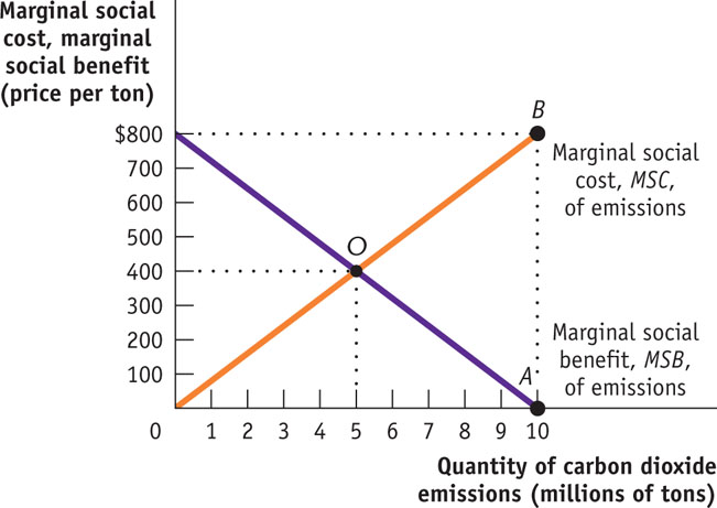
The optimal social quantity of pollution is at the point where the marginal social benefit of polluting equals the marginal social cost of polluting. As shown in the accompanying figure, this occurs at point O, the intersection of the marginal social cost curve and the marginal social benefit curve. At point O, the optimal quantity of emissions is 5 million tons and the marginal social benefit of emissions, which equals the marginal social cost of emissions, is $400 per ton. 
Find the market-determined quantity of pollution.
Review the section “Pollution: An External Cost” on pp. 277–279. In a market economy without government intervention to protect the environment, only the benefits of pollution are taken into account. Polluters will continue to pollute until there are no further benefits—when the marginal benefit of polluting is zero.
The market-determined quantity of pollution will be at the point where the marginal benefits to polluters are zero. As there are no marginal social benefits to pollution beyond the cost savings realized by the polluters themselves, the market-determined quantity will be at the point where the marginal social benefit of pollution is zero. This occurs at a carbon dioxide emissions level of 10 million tons, as shown at point A on the figure.
Find the social gain from reducing the quantity of pollution by one ton from the market-determined level.
Review the section “The Inefficiency of Excess Pollution” on p. 279. Find the marginal social cost of a ton of emissions at 10 million tons. Find the marginal social benefit of a ton of emissions at 10 million tons. The difference between these two numbers is the social gain.
Moving up from point A to point B in the figure, we can see that the marginal social cost of polluting at the market-determined level of 10 million tons is high at $800 per ton. The marginal social benefit at point A is zero. As the marginal cost per ton of polluting at a level of 10 million tons is $800 per ton and the marginal social benefit per ton of polluting at that level is zero, reducing the quantity of pollution by one ton leads to a net gain in total surplus of approximately $800 − 0 = $800.
301