Investment Spending
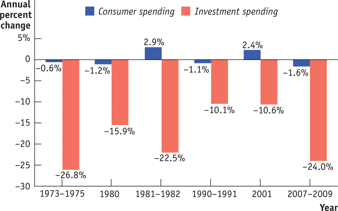
Although consumer spending is much larger than investment spending, booms and busts in investment spending tend to drive the business cycle. In fact, most recessions originate as a fall in investment spending. Figure 11-7 illustrates this point; it shows the annual percent change of investment spending and consumer spending in the United States, measured in real terms, during six recessions from 1973 to 2009. As you can see, swings in investment spending are much more dramatic than those in consumer spending. In addition, due to the multiplier process, economists believe that declines in consumer spending are usually the result of a process that begins with a slump in investment spending. Soon we’ll examine in more detail how a slump in investment spending generates a fall in consumer spending through the multiplier process.
Planned investment spending is the investment spending that businesses intend to undertake during a given period.
Before we do that, however, let’s analyze the factors that determine investment spending, which are somewhat different from those that determine consumer spending. The most important ones are the interest rate and expected future real GDP. We’ll also revisit a fact that we noted in Chapter 10: the level of investment spending businesses actually carry out is sometimes not the same level as planned investment spending, the investment spending that firms intend to undertake during a given period. Planned investment spending depends on three principal factors: the interest rate, the expected future level of real GDP, and the current level of production capacity. First, we’ll analyze the effect of the interest rate.
The Interest Rate and Investment Spending
Interest rates have their clearest effect on one particular form of investment spending: spending on residential construction—
Consider a potential home-
Interest rates also affect other forms of investment spending. Firms with investment spending projects will only go ahead with a project if they expect a rate of return higher than the cost of the funds they would have to borrow to finance that project. As we saw in Chapter 10, if the interest rate rises, fewer projects will pass that test, and as a result investment spending will be lower.
You might think that the trade-
So the trade-
So planned investment spending—
Expected Future Real GDP, Production Capacity, and Investment Spending
Suppose a firm has enough capacity to continue to produce the amount it is currently selling but doesn’t expect its sales to grow in the future. Then it will engage in investment spending only to replace existing equipment and structures that wear out or are rendered obsolete by new technologies. But if, instead, the firm expects its sales to grow rapidly in the future, it will find its existing production capacity insufficient for its future production needs. So the firm will undertake investment spending to meet those needs. This implies that, other things equal, firms will undertake more investment spending when they expect their sales to grow.
Now suppose that the firm currently has considerably more capacity than necessary to meet current production needs. Even if it expects sales to grow, it won’t have to undertake investment spending for a while—
If we put together the effects on investment spending of growth in expected future sales and the size of current production capacity, we can see one situation in which we can be reasonably sure that firms will undertake high levels of investment spending: when they expect sales to grow rapidly. In that case, even excess production capacity will soon be used up, leading firms to resume investment spending.
According to the accelerator principle, a higher growth rate of real GDP leads to higher planned investment spending, but a lower growth rate of real GDP leads to lower planned investment spending.
What is an indicator of high expected growth of future sales? It’s a high expected future growth rate of real GDP. A higher expected future growth rate of real GDP results in a higher level of planned investment spending, but a lower expected future growth rate of real GDP leads to lower planned investment spending. This relationship is summarized in a proposition known as the accelerator principle. As we explain in the upcoming Economics in Action, in 2006, when expectations of future real GDP growth turned negative, planned investment spending—
Inventories and Unplanned Investment Spending
Inventories are stocks of goods held to satisfy future sales.
Most firms maintain inventories, stocks of goods held to satisfy future sales. Firms hold inventories so they can quickly satisfy buyers—
Inventory investment is the value of the change in total inventories held in the economy during a given period.
As we explained in Chapter 7, a firm that increases its inventories is engaging in a form of investment spending. Suppose, for example, that the U.S. auto industry produces 800,000 cars per month but sells only 700,000. The remaining 100,000 cars are added to the inventory at auto company warehouses or car dealerships, ready to be sold in the future. Inventory investment is the value of the change in total inventories held in the economy during a given period. Unlike other forms of investment spending, inventory investment can actually be negative. If, for example, the auto industry reduces its inventory over the course of a month, we say that it has engaged in negative inventory investment.
To understand inventory investment, think about a manager stocking the canned goods section of a supermarket. The manager tries to keep the store fully stocked so that shoppers can almost always find what they’re looking for. But the manager does not want the shelves too heavily stocked because shelf space is limited and products can spoil. Similar considerations apply to many firms and typically lead them to manage their inventories carefully.
Unplanned inventory investment occurs when actual sales are more or less than businesses expected, leading to unplanned changes in inventories.
Actual investment spending is the sum of planned investment spending and unplanned inventory investment.
However, sales fluctuate. And because firms cannot always accurately predict sales, they often find themselves holding more or less inventories than they had intended. These unintended swings in inventories due to unforeseen changes in sales are called unplanned inventory investment. They represent investment spending, positive or negative, that occurred but was unplanned.
So in any given period, actual investment spending is equal to planned investment spending plus unplanned inventory investment. If we let IUnplanned represent unplanned inventory investment, IPlanned represent planned investment spending, and I represent actual investment spending, then the relationship among all three can be represented as:


To see how unplanned inventory investment can occur, let’s continue to focus on the auto industry and make the following assumptions. First, let’s assume that the industry must determine each month’s production volume in advance, before it knows the volume of actual sales. Second, let’s assume that it anticipates selling 800,000 cars next month and that it plans neither to add to nor subtract from existing inventories. In that case, it will produce 800,000 cars to match anticipated sales.
Now imagine that next month’s actual sales are less than expected, only 700,000 cars. As a result, the value of 100,000 cars will be added to investment spending as unplanned inventory investment.
The auto industry will, of course, eventually adjust to this slowdown in sales and the resulting unplanned inventory investment. It is likely that it will cut next month’s production volume in order to reduce inventories. In fact, economists who study macroeconomic variables in an attempt to determine the future path of the economy pay careful attention to changes in inventory levels. Rising inventories typically indicate positive unplanned inventory investment and a slowing economy, as sales are less than had been forecast. Falling inventories typically indicate negative unplanned inventory investment and a growing economy, as sales are greater than forecast. In the next section, we will see how production adjustments in response to fluctuations in sales and inventories ensure that the value of final goods and services actually produced is equal to desired purchases of those final goods and services.
ECONOMICS in Action: Interest Rates and the U.S. Housing Boom
Interest Rates and the U.S. Housing Boom
The housing boom in the Ft. Myers metropolitan area, described at the beginning of this chapter, was part of a broader housing boom in the country as a whole. There is little question that this housing boom was caused, in the first instance, by low interest rates.
Figure 11-8 shows the interest rate on 30-
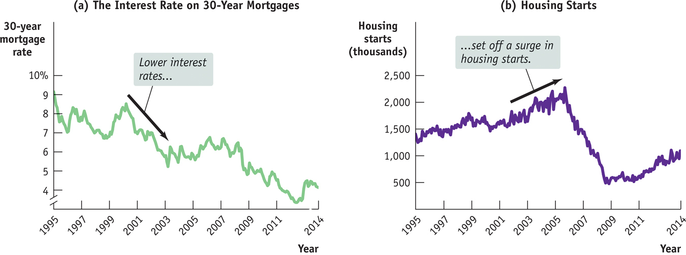
The low interest rates led to a large increase in residential investment spending, reflected in a surge of housing starts, shown in panel (b). This rise in investment spending drove an overall economic expansion, both through its direct effects and through the multiplier process.
Unfortunately, the housing boom eventually turned into too much of a good thing. By 2006, it was clear that the U.S. housing market was experiencing a bubble: people were buying housing based on unrealistic expectations about future price increases. When the bubble burst, housing—
Quick Review
Planned investment spending is negatively related to the interest rate and positively related to expected future real GDP. According to the accelerator principle, there is a positive relationship between planned investment spending and the expected future growth rate of real GDP.
Firms hold inventories to sell in the future. Inventory investment, a form of investment spending, can be positive or negative.
When actual sales are more or less than expected, unplanned inventory investment occurs. Actual investment spending is equal to planned investment spending plus unplanned inventory investment.
11-3
Question 11.6
For each event, explain whether planned investment spending or unplanned inventory investment will change and in what direction.
An unexpected increase in consumer spending
A sharp rise in the cost of business borrowing
A sharp increase in the economy’s growth rate of real GDP
An unanticipated fall in sales
Question 11.7
Historically, investment spending has experienced more extreme upward and downward swings than consumer spending. Why do you think this is so? (Hint: Consider the marginal propensity to consume and the accelerator principle.)
Question 11.8
Consumer spending was sluggish in late 2007, and economists worried that an inventory overhang—a high level of unplanned inventory investment throughout the economy—
would make it difficult for the economy to recover anytime soon. Explain why an inventory overhang might, like the existence of too much production capacity, depress current economic activity.
Solutions appear at back of book.