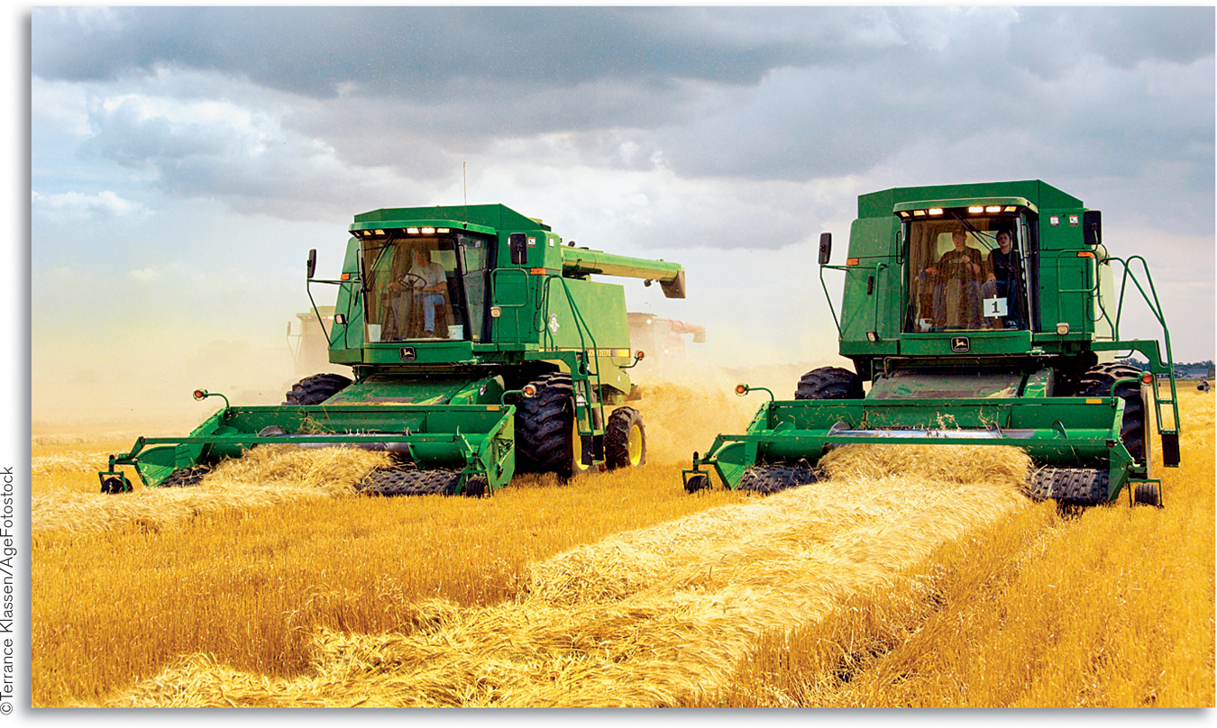
“O BEAUTIFUL FOR SPACIOUS (skies, for amber waves of grain.” So begins the song “America the Beautiful.” And those amber waves of grain are for real: though farmers are now only a small minority of America’s population, our agricultural industry is immensely productive and feeds much of the world.
If you look at agricultural statistics, however, something may seem a bit surprising: when it comes to yield per acre, U.S. farmers are often nowhere near the top. For example, farmers in Western European countries grow about three times as much wheat per acre as their U.S. counterparts. Are the Europeans better at growing wheat than we are?
No: European farmers are very skillful, but no more so than Americans. They produce more wheat per acre because they employ more inputs—more fertilizer and, especially, more labor—per acre. Of course, this means that European farmers have higher costs than their American counterparts. But because of government policies, European farmers receive a much higher price for their wheat than American farmers. This gives them an incentive to use more inputs and to expend more effort at the margin to increase the crop yield per acre.
Notice our use of the phrase “at the margin.” Like most decisions that involve a comparison of benefits and costs, decisions about inputs and production involve a comparison of marginal quantities—the marginal cost versus the marginal benefit of producing a bit more from each acre.
In Chapter 9 we considered the case of Alex, who had to choose the number of years of schooling that maximized his profit from schooling. There we used the profit-maximizing principle of marginal analysis to find the optimal quantity of years of schooling. In this chapter, we will encounter producers who have to make similar “how much” decisions: choosing the quantity of output produced to maximize profit.
Here and in Chapter 12, we will show how marginal analysis can be used to understand these output decisions—decisions that lie behind the supply curve. The first step in this analysis is to show how the relationship between a firm’s inputs and its output—its production function—determines its cost curves, the relationship between cost and quantity of output produced. That is what we do in this chapter. In Chapter 12, we will use our understanding of the firm’s cost curves to derive the individual and the market supply curves.