All economic decisions are about comparing costs and benefits—and usually about comparing marginal costs and marginal benefits. This goes both for a consumer, deciding whether to undertake another year of schooling, and for a producer, deciding whether to hire an additional worker.

Although there are some important exceptions, most factor markets in the modern American economy are perfectly competitive, meaning that buyers and sellers of a given factor are price-takers. And in a competitive labor market, it’s clear how to define an employer’s marginal cost of a worker: it is simply the worker’s wage rate. But what is the marginal benefit of that worker? To answer that question, we return to a concept first introduced in Chapter 11: the production function, which relates inputs to output. And as in Chapter 12, we will assume throughout this chapter that all producers are price-takers in their output markets—that is, they operate in a perfectly competitive industry.

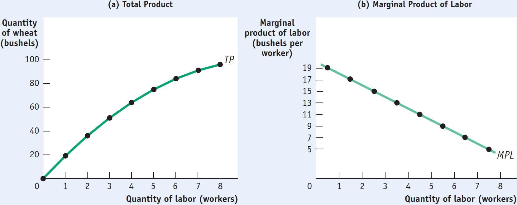
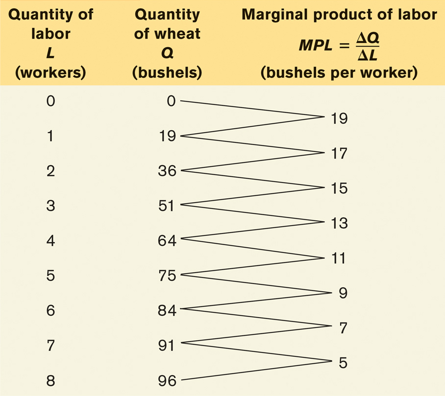
Figure 19-2 reproduces Figures 11-1 and 11-2, which showed the production function for wheat on George and Martha’s farm. Panel (a) uses the total product curve to show how total wheat production depends on the number of workers employed on the farm; panel (b) shows how the marginal product of labor, the increase in output from employing one more worker, depends on the number of workers employed. Table 19-1, which reproduces the table in Figure 11-1, shows the numbers behind the figure.

Assume that George and Martha want to maximize their profit, that workers must be paid $200 each, and that wheat sells for $20 per bushel. What is their optimal number of workers? That is, how many workers should they employ to maximize profit?

In Chapters 11 and 12 we showed how to answer this question in several steps. In Chapter 11 we used information from the producer’s production function to derive the firm’s total cost and its marginal cost. And in Chapter 12 we derived the price-taking firm’s optimal output rule: a price-taking firm’s profit is maximized by producing the quantity of output at which the marginal cost of the last unit produced is equal to the market price. Having determined the optimal quantity of output, we can go back to the production function and find the optimal number of workers—it is simply the number of workers needed to produce the optimal quantity of output.

There is, however, another way to use marginal analysis to find the number of workers that maximizes a producer’s profit. We can go directly to the question of what level of employment maximizes profit. This alternative approach is equivalent to the approach we outlined in the preceding paragraph—it’s just a different way of looking at the same thing. But it gives us more insight into the demand for factors as opposed to the supply of goods.

To see how this alternative approach works, let’s suppose that George and Martha are considering whether or not to employ an additional worker. The increase in cost from employing that additional worker is the wage rate, W. The benefit to George and Martha from employing that extra worker is the value of the extra output that worker can produce. What is this value? It is the marginal product of labor, MPL, multiplied by the price per unit of output, P. This amount—the extra value of output that is generated by employing one more unit of labor—is known as the value of the marginal product of labor, or VMPL:

(19-1) Value of the marginal product of labor = VMPL = P × MPL

So should George and Martha hire that extra worker? The answer is yes if the value of the extra output is more than the cost of the worker—that is, if VMPL > W. Otherwise they shouldn’t hire that worker.

So the decision to hire labor is a marginal decision, in which the marginal benefit to the producer from hiring an additional worker (VMPL) should be compared with the marginal cost to the producer (W). And as with any marginal decision, the optimal choice is where marginal benefit is just equal to marginal cost. That is, to maximize profit George and Martha will employ workers up to the point at which, for the last worker employed:

(19-2) VMPL = W at the profit-maximizing level of employment

This rule doesn’t apply only to labor; it applies to any factor of production. The value of the marginal product of any factor is its marginal product times the price of the good it produces. The general rule is that a profit-maximizing price-taking producer employs each factor of production up to the point at which the value of the marginal product of the last unit of the factor employed is equal to that factor’s price.

It’s important to realize that this rule doesn’t conflict with our analysis in Chapters 11 and 12. There we saw that a profit-maximizing producer of a good chooses the level of output at which the price of that good is equal to the marginal cost of production. It’s just a different way of looking at the same rule. If the level of output is chosen so that price equals marginal cost, then it is also true that at that output level the value of the marginal product of labor will equal the wage rate.

Now let’s look more closely at why choosing the level of employment at which the value of the marginal product of the last worker employed is equal to the wage rate works—and at how it helps us understand factor demand.

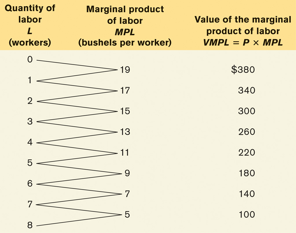
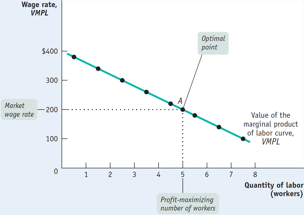
Table 19-2 calculates the value of the marginal product of labor on George and Martha’s farm, on the assumption that the price of wheat is $20 per bushel. In Figure 19-3 the horizontal axis shows the number of workers employed; the vertical axis measures the value of the marginal product of labor and the wage rate. The curve shown is the value of the marginal product curve of labor. This curve, like the marginal product of labor curve, slopes downward because of diminishing returns to labor in production. That is, the value of the marginal product of each worker is less than that of the preceding worker, because the marginal product of each worker is less than that of the preceding worker.

We have just seen that to maximize profit, George and Martha must hire workers up to the point at which the wage rate is equal to the value of the marginal product of the last worker employed. Let’s use the example to see how this principle really works.

Assume that George and Martha currently employ 3 workers and that workers must be paid the market wage rate of $200. Should they employ an additional worker?

Looking at Table 19-2, we see that if George and Martha currently employ 3 workers, the value of the marginal product of an additional worker is $260. So if they employ an additional worker, they will increase the value of their production by $260 but increase their cost by only $200, yielding an increased profit of $60. In fact, a producer can always increase total profit by employing one more unit of a factor of production as long as the value of the marginal product produced by that unit exceeds its factor price.

Alternatively, suppose that George and Martha employ 8 workers. By reducing the number of workers to 7, they can save $200 in wages. In addition, the value of the marginal product of the last one, the 8th worker, was only $100. So, by reducing employment by one worker, they can increase profit by $200 − $100 = $100. In other words, a producer can always increase total profit by employing one less unit of a factor of production as long as the value of the marginal product produced by that unit is less than the factor price.

Using this method, we can see from Table 19-2 that the profit-maximizing employment level is 5 workers given a wage rate of $200. The value of the marginal product of the 5th worker is $220, so adding the 5th worker results in $20 of additional profit. But George and Martha should not hire more than 5 workers: the value of the marginal product of the 6th worker is only $180, $20 less than the cost of that worker. So, to maximize total profit, George and Martha should employ workers up to but not beyond the point at which the value of the marginal product of the last worker employed is equal to the wage rate.

Now look again at the value of the marginal product curve in Figure 19-3. To determine the profit-maximizing level of employment, we set the value of the marginal product of labor equal to the price of labor—a wage rate of $200 per worker. This means that the profit-maximizing level of employment is at point A, corresponding to an employment level of 5 workers. If the wage rate were higher than $200, we would simply move up the curve and reduce the number of workers employed; if the wage rate were lower than $200, we would move down the curve and increase the number of workers employed.

In this example, George and Martha have a small farm in which the potential employment level varies from 0 to 8 workers, and they hire workers up to the point at which the value of the marginal product of the last worker is greater than or equal to the wage rate. (To go beyond this point and hire workers for which the wage exceeds the value of the marginal product would reduce George and Martha’s profit.)

Suppose, however, that the firm in question is large and has the potential of hiring many workers. When there are many employees, the value of the marginal product of labor falls only slightly when an additional worker is employed. As a result, there will be some worker whose value of the marginal product almost exactly equals the wage rate. (In keeping with the George and Martha example, this means that some worker generates a value of the marginal product of approximately $200.) In this case, the firm maximizes profit by choosing a level of employment at which the value of the marginal product of the last worker hired equals (to a very good approximation) the wage rate.

In the interest of simplicity, we will assume from now on that firms use this rule to determine the profit-maximizing level of employment. This means that the value of the marginal product of labor curve is the individual producer’s labor demand curve. And, in general, a producer’s value of the marginal product curve for any factor of production is that producer’s individual demand curve for that factor of production.

As in the case of ordinary demand curves, it is important to distinguish between movements along the factor demand curve and shifts of the factor demand curve. What causes factor demand curves to shift? There are three main causes:

1. Changes in Price of Output Remember that factor demand is derived demand: if the price of the good that is produced with a factor changes, so will the value of the marginal product of the factor. That is, in the case of labor demand, if P changes, VMPL = P × MPL will change at any given level of employment.

Figure 19-4 illustrates the effects of changes in the price of wheat, assuming that $200 is the current wage rate. Panel (a) shows the effect of an increase in the price of wheat. This shifts the value of the marginal product of labor curve upward, because VMPL rises at any given level of employment. If the wage rate remains unchanged at $200, the optimal point moves from point A to point B: the profit-maximizing level of employment rises.

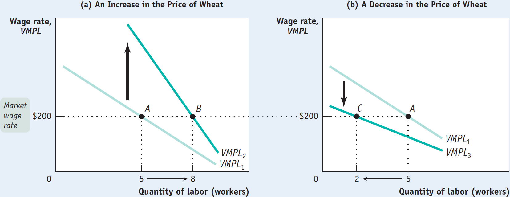
Panel (b) shows the effect of a decrease in the price of wheat. This shifts the value of the marginal product of labor curve downward. If the wage rate remains unchanged at $200, the optimal point moves from point A to point C: the profit-maximizing level of employment falls.

2. Changes in Supply of Other Factors Suppose that George and Martha acquire more land to cultivate—say, by clearing a woodland on their property. Each worker now produces more wheat because each one has more land to work with. As a result, the marginal product of labor on the farm rises at any given level of employment. This has the same effect as an increase in the price of wheat, which is illustrated in panel (a) of Figure 19-4: the value of the marginal product of labor curve shifts upward, and at any given wage rate the profit-maximizing level of employment rises.

In contrast, suppose George and Martha cultivate less land. This leads to a fall in the marginal product of labor at any given employment level. Each worker produces less wheat because each has less land to work with. As a result, the value of the marginal product of labor curve shifts downward—as in panel (b) of Figure 19-4—and the profit-maximizing level of employment falls.

3. Changes in Technology In general, the effect of technological progress on the demand for any given factor can go either way: improved technology can either increase or reduce the demand for a given factor of production.

How can technological progress reduce factor demand? Consider horses, which were once an important factor of production. The development of substitutes for horse power, such as automobiles and tractors, greatly reduced the demand for horses.

The usual effect of technological progress, however, is to increase the demand for a given factor by raising its productivity. So despite persistent fears that machinery would reduce the demand for labor, over the long run the U.S. economy has seen both large wage increases and large increases in employment. That’s because technological progress has raised labor productivity, and as a result increased the demand for labor.

We’ve now seen that each perfectly competitive producer in a perfectly competitive factor market maximizes profit by hiring labor up to the point at which its value of the marginal product is equal to its price—in the case of labor, to the point where VMPL = W. What does this tell us about labor’s share in the factor distribution of income? To answer that question, we need to examine equilibrium in the labor market. From that vantage point we will go on to learn about the markets for land and capital and about how they also influence the factor distribution of income.

Let’s start by assuming that the labor market is in equilibrium: at the current market wage rate, the number of workers that producers want to employ is equal to the number of workers willing to work. Thus, all employers pay the same wage rate, and each employer, whatever he or she is producing, employs labor up to the point at which the value of the marginal product of the last worker hired is equal to the market wage rate.

This situation is illustrated in Figure 19-5, which shows the value of the marginal product curves of two producers—Farmer Jones, who produces wheat, and Farmer Smith, who produces corn. Despite the fact that they produce different products, they compete for the same workers and so must pay the same wage rate, $200. When both farmers maximize profit, both hire labor up to the point at which its value of the marginal product is equal to the wage rate. In the figure, this corresponds to employment of 5 workers by Jones and 7 by Smith.

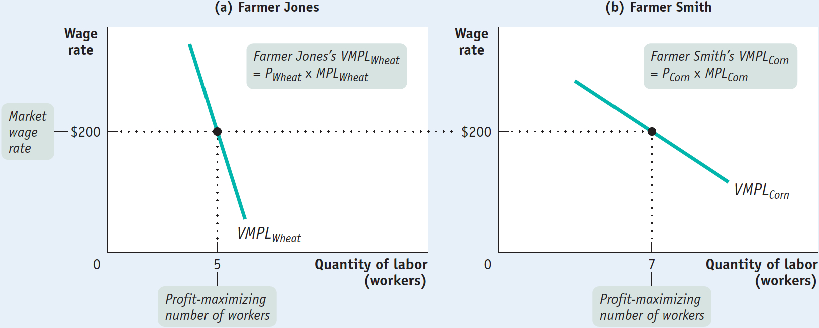
Figure 19-6 illustrates the labor market as a whole. The market labor demand curve, like the market demand curve for a good (shown in Figure 3-5), is the horizontal sum of all the individual labor demand curves of all the producers who hire labor. And recall that each producer’s individual labor demand curve is the same as his or her value of the marginal product of labor curve.

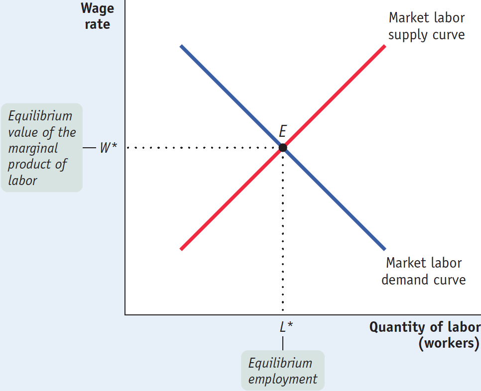
For now, let’s simply assume an upward-sloping labor supply curve; we’ll discuss labor supply later in this chapter. Then the equilibrium wage rate is the wage rate at which the quantity of labor supplied is equal to the quantity of labor demanded. In Figure 19-6, this leads to an equilibrium wage rate of W* and the corresponding equilibrium employment level of L*. (The equilibrium wage rate is also known as the market wage rate.)

And as we showed in the examples of the farms of George and Martha and of Farmer Jones and Farmer Smith (where the equilibrium wage rate is $200), each farm hires labor up to the point at which the value of the marginal product of labor is equal to the equilibrium wage rate. Therefore, in equilibrium, the value of the marginal product of labor is the same for all employers. So the equilibrium (or market) wage rate is equal to the equilibrium value of the marginal product of labor—the additional value produced by the last unit of labor employed in the labor market as a whole. It doesn’t matter where that additional unit is employed, since equilibrium VMPL is the same for all producers.

What we have just learned, then, is that the market wage rate is equal to the equilibrium value of the marginal product of labor. And the same is true of each factor of production: in a perfectly competitive market economy, the market price of each factor is equal to its equilibrium value of the marginal product. Let’s examine the markets for land and (physical) capital now. (From this point on, we’ll refer to physical capital as simply “capital.”)

If we maintain the assumption that the markets for goods and services are perfectly competitive, the result that we derived for the labor market also applies to other factors of production. Suppose, for example, that a farmer is considering whether to rent an additional acre of land for the next year. He or she will compare the cost of renting that acre with the value of the additional output generated by employing an additional acre—the value of the marginal product of an acre of land. To maximize profit, the farmer must employ land up to the point at which the value of the marginal product of an acre of land is equal to the rental rate per acre.

What if the farmer already owns the land? We already saw the answer in Chapter 9, which dealt with economic decisions: even if you own land, there is an implicit cost—the opportunity cost—of using it for a given activity, because it could be used for something else, such as renting it out to other farmers at the market rental rate. So a profit-maximizing producer employs additional acres of land up to the point at which the cost of the last acre employed, explicit or implicit, is equal to the value of the marginal product of that acre.

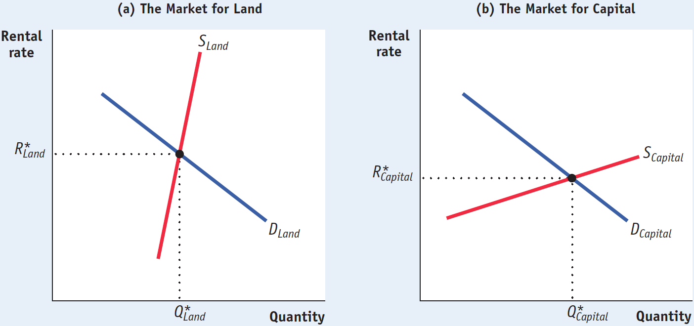
The same is true for capital. The explicit or implicit cost of using a unit of land or capital for a set period of time is called its rental rate. In general, a unit of land or capital is employed up to the point at which that unit’s value of the marginal product is equal to its rental rate over that time period. How are the rental rates for land and capital determined? By the equilibria in the land market and the capital market, of course. Figure 19-7 illustrates those outcomes.

Panel (a) shows the equilibrium in the market for land. Summing over the individual demand curves for land of all producers gives us the market demand curve for land. Due to diminishing returns, the demand curve slopes downward, like the demand curve for labor. As we have drawn it, the supply curve of land is relatively steep and therefore relatively inelastic. This reflects the fact that finding new supplies of land for production is typically difficult and expensive—for example, creating new farmland through expensive irrigation. The equilibrium rental rate for land, , and the equilibrium quantity of land employed in production, , are given by the intersection of the two curves.

Panel (b) shows the equilibrium in the market for capital. In contrast to the supply curve for land, the supply curve for capital is relatively elastic. That’s because the supply of capital is relatively responsive to price: capital is paid for with funds that come from the savings of investors, and the amount of savings that investors make available is relatively responsive to the rental rate for capital. The equilibrium rental rate for capital, , and the equilibrium quantity of capital employed in production, , are given by the intersection of the two curves.

So we have learned that when the markets for goods and services and the factor markets are perfectly competitive, a factor of production will be employed up to the point at which its value of the marginal product is equal to its market equilibrium price. That is, it will be paid its equilibrium value of the marginal product. What does this say about the factor distribution of income? It leads us to the marginal productivity theory of income distribution, which says that each factor is paid the value of the output generated by the last unit of that factor employed in the factor market as a whole—its equilibrium value of the marginal product.

To understand why the marginal productivity theory of income distribution is important, look back at Figure 19-1, which shows the factor distribution of income in the United States, and ask yourself this question: who or what decided that labor would get 66% of total U.S. income? Why not 90% or 50%?

The answer, according to the marginal productivity theory of income distribution, is that the division of income among the economy’s factors of production isn’t arbitrary: it is determined by each factor’s marginal productivity at the economy’s equilibrium. The wage rate earned by all workers in the economy is equal to the increase in the value of output generated by the last worker employed in the economy-wide labor market.

Here we have assumed that all workers are of the same ability. (Similarly, we’ve assumed that all units of land and capital are equally productive.) But in reality workers differ considerably in ability.

Rather than thinking of one labor market for all workers in the economy, we can instead think of different markets for different types of workers, where workers are of equivalent ability within each market. For example, the market for computer programmers is different from the market for pastry chefs.

In the market for computer programmers, all participants are assumed to have equal ability; likewise for the market for pastry chefs. In this scenario, the marginal productivity theory of income distribution still holds. That is, when the labor market for computer programmers is in equilibrium, the wage rate earned by all computer programmers is equal to the market’s equilibrium value of the marginal product—the value of the marginal product of the last computer programmer hired in that market.