The Supply of Labor
Up to this point we have focused on the demand for factors, which determines the quantities demanded of labor, capital, or land by producers as a function of their factor prices. What about the supply of factors?
In this section we focus exclusively on the supply of labor. We do this for two reasons. First, in the modern U.S. economy, labor is the most important factor of production, accounting for most of factor income. Second, as we’ll see, labor supply is the area in which factor markets look most different from markets for goods and services.
Work versus Leisure
In the labor market, the roles of firms and households are the reverse of what they are in markets for goods and services. A good such as wheat is supplied by firms and demanded by households; labor, though, is demanded by firms and supplied by households. How do people decide how much labor to supply?
As a practical matter, most people have limited control over their work hours: either you take a job that involves working a set number of hours per week, or you don’t get the job at all. To understand the logic of labor supply, however, it helps to put realism to one side for a bit and imagine an individual who can choose to work as many or as few hours as he or she likes.

Decisions about labor supply result from decisions about time allocation: how many hours to spend on different activities.
Why wouldn’t such an individual work as many hours as possible? Because workers are human beings, too, and have other uses for their time. An hour spent on the job is an hour not spent on other, presumably more pleasant, activities. So the decision about how much labor to supply involves making a decision about time allocation—how many hours to spend on different activities.
Leisure is time available for purposes other than earning money to buy marketed goods.
By working, people earn income that they can use to buy goods. The more hours an individual works, the more goods he or she can afford to buy. But this increased purchasing power comes at the expense of a reduction in leisure, the time spent not working. (Leisure doesn’t necessarily mean time spent goofing off. It could mean time spent with one’s family, pursuing hobbies, exercising, and so on.) And though purchased goods yield utility, so does leisure. Indeed, we can think of leisure itself as a normal good, which most people would like to consume more of as their incomes increase.
How does a rational individual decide how much leisure to consume? By making a marginal comparison, of course. In analyzing consumer choice, we asked how a utility-
Consider Clive, an individual who likes both leisure and the goods money can buy. Suppose that his wage rate is $10 per hour. In deciding how many hours he wants to work, he must compare the marginal utility of an additional hour of leisure with the additional utility he gets from $10 worth of goods. If $10 worth of goods adds more to his total utility than an additional hour of leisure, he can increase his total utility by giving up an hour of leisure in order to work an additional hour. If an extra hour of leisure adds more to his total utility than $10 worth of goods, he can increase his total utility by working one fewer hour in order to gain an hour of leisure.
At Clive’s optimal labor supply choice, then, his marginal utility of one hour of leisure is equal to the marginal utility he gets from the goods that his hourly wage can purchase. This is very similar to the optimal consumption rule we encountered in Chapter 10, except that it is a rule about time rather than money.
Our next step is to ask how Clive’s decision about time allocation is affected when his wage rate changes.
Wages and Labor Supply
Suppose that Clive’s wage rate doubles, from $10 to $20 per hour. How will he change his time allocation?
You could argue that Clive will work longer hours, because his incentive to work has increased: by giving up an hour of leisure, he can now gain twice as much money as before. But you could equally well argue that he will work less, because he doesn’t need to work as many hours to generate the income to pay for the goods he wants.
As these opposing arguments suggest, the quantity of labor Clive supplies can either rise or fall when his wage rate rises. To understand why, let’s recall the distinction between substitution effects and income effects that we learned in Chapter 10 and its appendix. We saw there that a price change affects consumer choice in two ways: by changing the opportunity cost of a good in terms of other goods (the substitution effect) and by making the consumer richer or poorer (the income effect).
Now think about how a rise in Clive’s wage rate affects his demand for leisure. The opportunity cost of leisure—
So in the case of labor supply, the substitution effect and the income effect work in opposite directions. If the substitution effect is so powerful that it dominates the income effect, an increase in Clive’s wage rate leads him to supply more hours of labor. If the income effect is so powerful that it dominates the substitution effect, an increase in the wage rate leads him to supply fewer hours of labor.
The individual labor supply curve shows how the quantity of labor supplied by an individual depends on that individual’s wage rate.
We see, then, that the individual labor supply curve—the relationship between the wage rate and the number of hours of labor supplied by an individual worker—
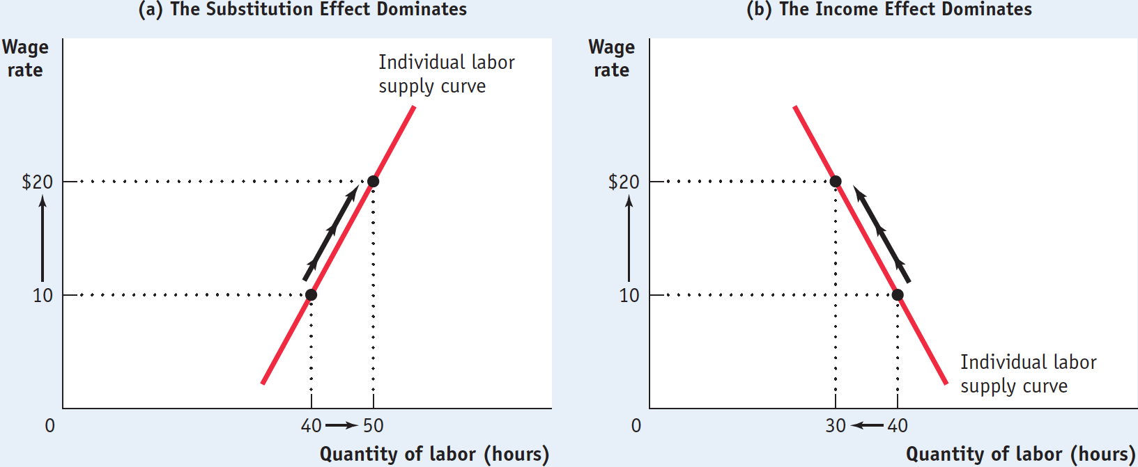
Figure 19-11 illustrates the two possibilities for labor supply. If the substitution effect dominates the income effect, the individual labor supply curve slopes upward; panel (a) shows an increase in the wage rate from $10 to $20 per hour leading to a rise in the number of hours worked from 40 to 50. However, if the income effect dominates, the quantity of labor supplied goes down when the wage rate increases. Panel (b) shows the same rise in the wage rate leading to a fall in the number of hours worked from 40 to 30. (Economists refer to an individual labor supply curve that contains both upward-
Is a negative response of the quantity of labor supplied to the wage rate a real possibility? Yes: many labor economists believe that income effects on the supply of labor may be somewhat stronger than substitution effects. The most compelling piece of evidence for this belief comes from Americans’ increasing consumption of leisure over the past century. At the end of the nineteenth century, wages adjusted for inflation were only about one-
FOR INQUIRING MINDS: Why You Can’t Find a Cab When It’s Raining
Everyone says that you can’t find a taxi in New York when you really need one—
When it’s raining, drivers get more fares and therefore earn more per hour. But it seems that the income effect of this higher wage rate outweighs the substitution effect.
This behavior led the authors of the study to question drivers’ rationality. They point out that if taxi drivers thought in terms of the long run, they would realize that rainy days and nice days tend to average out and that their high earnings on a rainy day don’t really affect their long-
Indeed, experienced drivers (who have probably figured this out) are less likely than inexperienced drivers to go home early on a rainy day. But leaving such issues to one side, the study does seem to show clear evidence of a labor supply curve that slopes downward instead of upward, thanks to income effects.
These findings give us a deeper understanding of the economics behind the spectacular rise of Uber, the company that matches passengers with available drivers for hire via a smartphone app. The fact that taxi drivers tend to head home just when people really need a ride has provided an opportunity for Uber: by allowing its drivers to charge more when demand shifts outward (a practice called surge pricing), Uber puts more drivers on the road despite the income effects on taxi drivers’ labor supply curves.
Shifts of the Labor Supply Curve
Now that we have examined how income and substitution effects shape the individual labor supply curve, we can turn to the market labor supply curve. In any labor market, the market supply curve is the horizontal sum of the individual labor supply curves of all workers in that market. A change in any factor other than the wage that alters workers’ willingness to supply labor causes a shift of the labor supply curve. A variety of factors can lead to such shifts, including changes in preferences and social norms, changes in population, changes in opportunities, and changes in wealth.
Changes in Preferences and Social Norms Changes in preferences and social norms can lead workers to increase or decrease their willingness to work at any given wage. A striking example of this phenomenon is the large increase in the number of employed women—
Changes in Population Changes in the population size generally lead to shifts of the labor supply curve. A larger population tends to shift the labor supply curve rightward as more workers are available at any given wage; a smaller population tends to shift the labor supply curve leftward. From 1990 to 2008, the U.S. labor force has grown approximately 1% per year, generated by immigration and a relatively high birth rate. As a result, from 1990 to 2008 the U.S. labor market had a rightward-
The Overworked American?
Americans today may work less than they did a hundred years ago, but they still work more than workers in any other industrialized country.
This figure compares average annual hours worked in the United States with those worked in other industrialized countries. The differences result from a combination of Americans’ longer workweeks and shorter vacations. For example, the great majority of full-
In 2013, American workers got, on average, eight paid vacation days, but 23% of American workers got none at all. In contrast, German workers are guaranteed six weeks of paid vacation a year. Also, American workers use fewer of the vacation days they are entitled to than do workers in other industrialized countries. A 2013 survey found that American workers used only 51% of the vacation days they are entitled to, compared to 90% in France.
Why do Americans work so much more than others? Unlike their counterparts in other industrialized countries, Americans are not legally entitled to paid vacation days; as a result, the average American worker gets fewer of them.
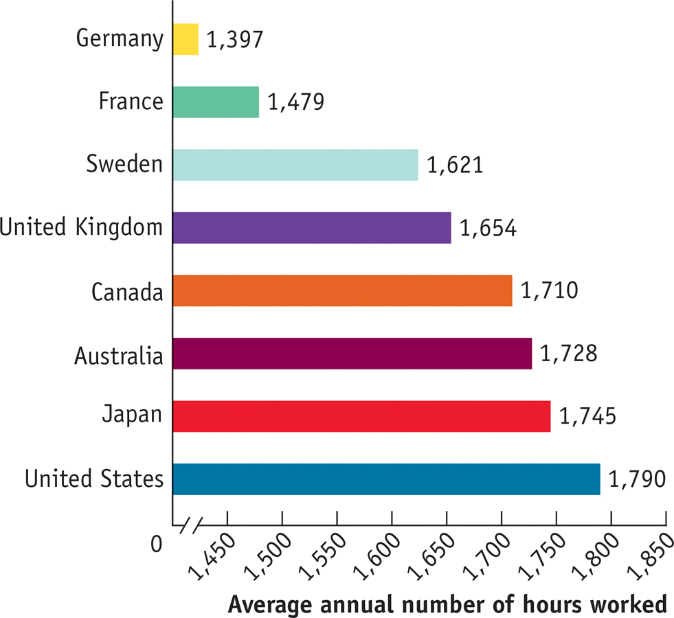
Source: OECD.
Changes in Opportunities At one time, teaching was the only occupation considered suitable for well-
Changes in Wealth A person whose wealth increases will buy more normal goods, including leisure. So when a class of workers experiences a general rise in their wealth levels—
!worldview! ECONOMICS in Action: The Decline of the Summer Job
The Decline of the Summer Job
Come summertime, resort towns along the New Jersey shore find themselves facing a recurring annual problem: a serious shortage of lifeguards. Traditionally, lifeguard positions, together with many other seasonal jobs, had been filled mainly by high school and college students. But in recent years a combination of adverse shifts in supply and demand have severely diminished summer employment for young workers. In 1979, 71% of Americans between the ages of 16 and 19 were in the summer workforce. By 2007, that number was 50%, and by 2013 it had taken another sharp fall to around 43%.

A fall in supply is one explanation for the change. More students now feel that they should devote their summer to additional study rather than to work. An increase in household affluence over the past 20 years has also contributed to fewer teens taking jobs because they no longer feel pressured to contribute to household finances. In other words, the income effect has led to a reduced labor supply.
Another explanation is the substitution effect: increased competition from immigrants, who are now doing the jobs typically done by teens (like mowing lawns and delivering pizzas), has led to a decline in wages. So many teenagers have forgone summer work to consume leisure instead.
But it was the deep recession of 2007-
Quick Review
The choice of how much labor to supply is a problem of time allocation: a choice between work and leisure.
A rise in the wage rate causes both an income and a substitution effect on an individual’s labor supply. The substitution effect of a higher wage rate induces more hours of work supplied, other things equal. This is countered by the income effect: higher income leads to a higher demand for leisure, a normal good. If the income effect dominates, a rise in the wage rate can actually cause the individual labor supply curve to slope the “wrong” way: downward.
The market labor supply curve is the horizontal sum of the individual labor supply curves of all workers in that market. It shifts for four main reasons: changes in preferences and social norms, changes in population, changes in opportunities, and changes in wealth.
19-4
Question 19.7
Formerly, Clive was free to work as many or as few hours per week as he wanted. But a new law limits the maximum number of hours he can work per week to 35. Explain under what circumstances, if at all, he is made:
Worse off
Equally as well off
Better off
Question 19.8
Explain in terms of the income and substitution effects how a fall in Clive’s wage rate can induce him to work more hours than before.
Solutions appear at back of book.
Wages and Workers at Costco and Walmart
In July 2013 President Barack Obama gave a much anticipated and widely discussed speech on the economy, arguing for policies that would raise wages and reduce income inequality. Along the way, he name-

Indeed, that same year, a Bloomberg BusinessWeek story about Costco reported that it paid an average wage of $20.89 an hour, compared with $12.67 at Walmart, and provided much more generous health benefits too. Despite paying much higher wages, however, Costco has been substantially more profitable than Walmart in recent years. How is this possible?
According to Costco executives, what they get in return for relatively high wages is a stable and highly productive workforce. Retail companies typically have high labor turnover—
Would Walmart be more profitable if it paid like Costco? Skeptics argue that the retailers aren’t completely comparable: Costco offers a narrower range of products and caters to a higher-
QUESTIONS FOR THOUGHT
Question 19.9
EL/VXz+SB7InYW3bC+R3kCtIdV0d/Vt6tDrV/BkmPGmugnbEvVrFXEU4tDmLC0ZSCecxv9HG4rnQsss0bPAvia0FUaRqzQqG6atbeT7cyiRHeVQvrVo7Kgd/K8POSP3Y4hI9QJ9nJYXQGJRgZFqMeBAaxkCRqC88hZttwK6yOSP1bgBaRb/J9RQCaAi/EVHNQQzwhYz322N1sass9AbY44fpn0KfnLNEUse the marginal productivity theory of income distribution to explain how companies like Walmart can pay workers so little that they fall below the poverty line.Question 19.10
tkH5zg/xZS80Wiuy/1u5dc6Sup8Cj6QwJuW7/EXex+20iqqepFkoLuue0mNYg68XPbRcnE14VvW0N3+Gox9E/s4w7XaPUT9F0qx28yBAPN8J4Dh9g6QLswMvmHjqgIbYJ5kIPOoF48oEcvhWZHt86Uu2J551ROFqWHjrtQ==How does the Costco story fit into our discussion of the reasons similar workers may end up being paid different wages?Question 19.11
1WcUjx1KeTcSlsqEkfK0Zx2QnlKJn993PRTxacY8+zKQ0xBjfzIvvls7kvK6DxhWNiQVM1oZlrkG8AbAXdClqU+HyqnXm09vIAjKThgopAFuGPJMyC1diCdMDpatKWK4ivVKDlok2q/pG/mhyFcd2CuOQwwU8kKibiyBKa5pdPt8dU48/RzRFQ16hn8DskFidEzrz0IMHp7mJfVHQhNUj8rFe8PoWVW0JSM4wlyX9JseI5RjScGSBEsiy3Frq7lyp7ODMX0oq0gS8vGcNjLjxud3Vd6wO7SYVeUP1JGdPfdzvkJS1Wbmzn+LcO8D6+ZE//cDIZ+wwdkikMyj5kOAyncJhVlTqzbA4IMVr94Jr6A1cCaa0NiVch6Yqx7PiKeZgJfXLiKo8CcAp/stNzKQvg==President Obama, as his speech indicated, would like to encourage more companies to adopt a high-wage strategy. Other politicians would like to do the same. What are the possible positive and negative effects if this becomes official government policy?