In the appendix to Chapter 10, we showed that consumer choice can be represented using the concept of indifference curves, which provide a “map” of consumer preferences. If you have covered the appendix, you may find it interesting to learn that indifference curves are also useful for addressing the issue of labor supply. In fact, this is one place where they are particularly helpful.

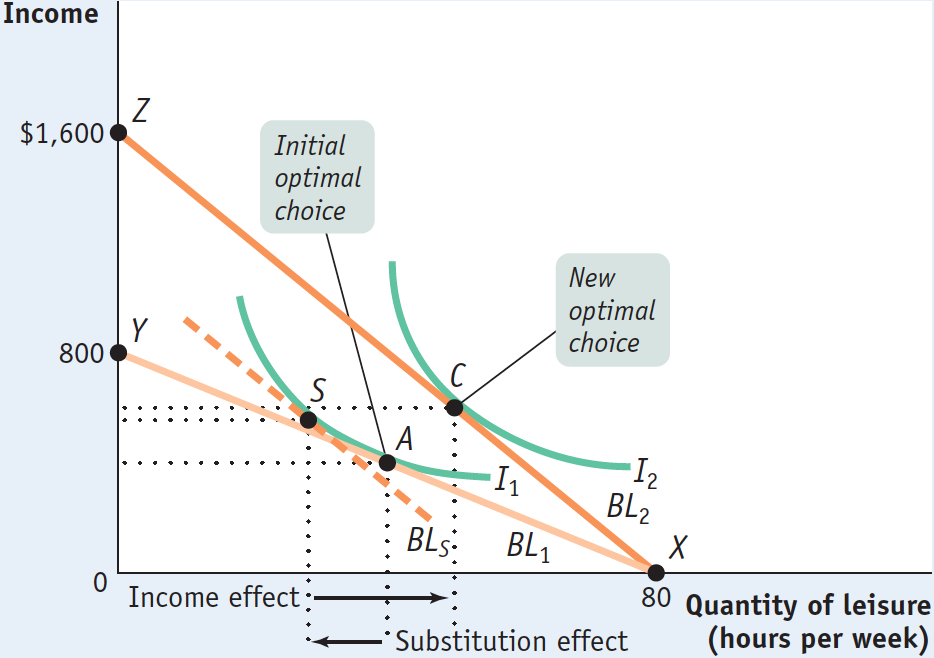
Using indifference curves, Figure 19A-4 shows how an increase in the wage rate can lead to a fall in the quantity of labor supplied. Point A is Clive’s initial optimal choice, given an hourly wage rate of $10. It is the same as point A in Figure 19A-1; this time, however, we include an indifference curve to show that it is a point at which the budget line is tangent to the highest possible indifference curve.

Now consider the effect of a rise in the wage rate to $20. Imagine, for a moment, that at the same time Clive was offered a higher wage, he was told that he had to start repaying his student loan and that the good-news/bad-news combination left his utility unchanged. Then he would find himself at point S: on the same indifference curve as at A, but tangent to a steeper budget line, the dashed line BL_s in Figure 19A-4, which is parallel to BL₂. The move from point A to point S is the substitution effect of his wage increase: it leads him to consume less leisure and therefore supply more labor.

But now cancel the repayment on the student loan, and Clive is able to move to a higher indifference curve. His new optimum is at point C, which corresponds to C in panel (b) of Figure 19A-2. The move from point S to point C is the income effect of his wage increase. And we see that this income effect can outweigh the substitution effect: at C he consumes more leisure, and therefore supplies less labor, than he did at A.