1.1 Module 83: History and Alternative Views of Macroeconomics

© Minnesota HistoricalSociety/CORBIS
Thomas W. Elliott

Classical Macroeconomics

The term macroeconomics appears to have been coined in 1933 by the Norwegian economist Ragnar Frisch. The timing, during the worst year of the Great Depression, was no accident. Still, there were economists analyzing what we now consider macroeconomic issues—the behavior of the aggregate price level and aggregate output—before then.

Money and the Price Level

Previously, we described the classical model of the price level. According to the classical model, prices are flexible, making the aggregate supply curve vertical even in the short run. In this model, an increase in the money supply leads, other things equal, to a proportional rise in the aggregate price level, with no effect on aggregate output. As a result, increases in the money supply lead to inflation, and that’s all. Before the 1930s, the classical model of the price level dominated economic thinking about the effects of monetary policy.

Did classical economists really believe that changes in the money supply affected only aggregate prices, without any effect on aggregate output? Probably not. Historians of economic thought argue that before 1930 most economists were aware that changes in the money supply affected aggregate output as well as aggregate prices in the short run—or, to use modern terms, they were aware that the short-run aggregate supply curve sloped upward. But they regarded such short-run effects as unimportant, stressing the long run instead. It was this attitude that led John Maynard Keynes to scoff at the focus on the long run, in which, as he said, “we are all dead.”

The Business Cycle

Classical economists were, of course, also aware that the economy did not grow smoothly. The American economist Wesley Mitchell pioneered the quantitative study of business cycles. In 1920, he founded the National Bureau of Economic Research, an independent, nonprofit organization that to this day has the official role of declaring the beginnings of recessions and expansions. Thanks to Mitchell’s work, the measurement of business cycles was well advanced by 1930. But there was no widely accepted theory of business cycles.

In the absence of any clear theory, views about how policy makers should respond to a recession were conflicting. Some economists favored expansionary monetary and fiscal policies to fight a recession. Others believed that such policies would worsen the slump or merely postpone the inevitable. When the Great Depression hit, the policy making process was paralyzed by this lack of consensus. In many cases, economists now believe, policy makers took steps in the wrong direction.

Necessity was, however, the mother of invention. As we’ll explain next, the Great Depression provided a strong incentive for economists to develop theories that could serve as a guide to policy—and economists responded.

The Great Depression and the Keynesian Revolution

The Great Depression demonstrated, once and for all, that economists cannot safely ignore the short run. Not only was the economic pain severe, it threatened to destabilize societies and political systems.

The whole world wanted to know how this economic disaster could be happening and what should be done about it. But because there was no widely accepted theory of the business cycle, economists gave conflicting and, we now believe, often harmful advice. Some believed that only a huge change in the economic system—such as having the government take over much of private industry and replace markets with a command economy—could end the slump. Others argued that slumps were natural—even beneficial—and that nothing should be done.

Some people use Keynesian economics as a synonym for left-wing economics—but, in truth, Keynes’s ideas have been accepted across a broad part of the political spectrum.

Tim Gidal/Picture Post/Getty Images

Some economists, however, argued that the slump both could have and should have been cured—without giving up on the basic idea of a market economy. In 1930, the British economist John Maynard Keynes compared the problems of the U.S. and British economies to those of a car with a defective alternator. Getting the economy running, he argued, would require only a modest repair, not a complete overhaul.

Nice metaphor. But what was the nature of the trouble?

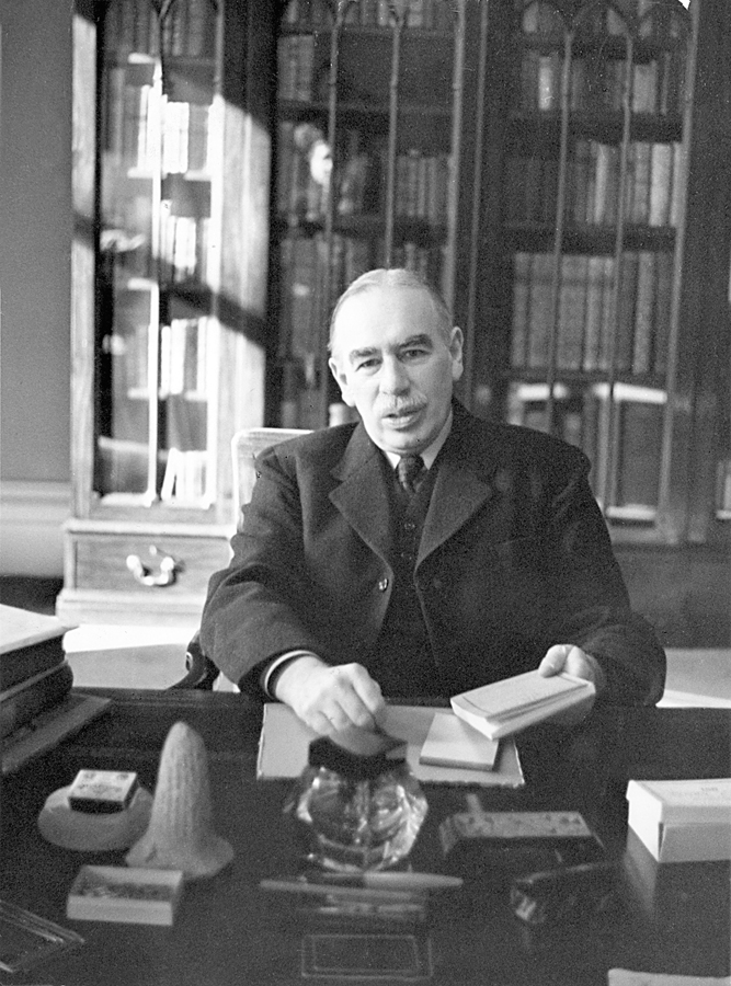
Keynes’s Theory

In 1936, Keynes presented his analysis of the Great Depression—his explanation of what was wrong with the economy’s alternator—in a book titled The General Theory of Employment, Interest, and Money. The General Theory stands with Adam Smith’s The Wealth of Nations as one of the most influential books on economics ever written.

Keynes’s book is a vast stew of ideas. And Keynesian economics mainly reflected two innovations. First, Keynes emphasized the short-run effects of shifts in aggregate demand on aggregate output, rather than the long-run determination of the aggregate price level. As Keynes’s famous remark about being dead in the long run suggests, until his book appeared most economists had treated short-run macroeconomics as a minor issue. Keynes focused the attention of economists on situations in which the short-run aggregate supply curve slopes upward and shifts in the aggregate demand curve affect aggregate output and employment as well as aggregate prices.

Figure 83-1 illustrates the difference between Keynesian and classical macroeconomics. Both panels of the figure show the short-run aggregate supply curve, SRAS; in both it is assumed that for some reason the aggregate demand curve shifts leftward from AD₁ to AD₂—let’s say in response to a fall in stock market prices that leads households to reduce consumer spending.

One important difference between classical and Keynesian economics involves the short-run aggregate supply curve. Panel (a) shows the classical view: the SRAS curve is vertical, so shifts in aggregate demand affect the aggregate price level but not aggregate output. Panel (b) shows the Keynesian view: in the short run the SRAS curve slopes upward, so shifts in aggregate demand affect aggregate output as well as aggregate prices.

Panel (a) shows the classical view: the short-run aggregate supply curve is vertical. The decline in aggregate demand leads to a fall in the aggregate price level, from P₁ to P₂, but no change in aggregate output. Panel (b) shows the Keynesian view: the short-run aggregate supply curve slopes upward, so the decline in aggregate demand leads to both a fall in the aggregate price level, from P₁ to P₂, and a fall in aggregate output, from Y₁ to Y₂.

As we’ve already explained, many classical macroeconomists would have agreed that panel (b) was an accurate story in the short run—but they regarded the short run as unimportant. Keynes disagreed. (Just to be clear, there isn’t any diagram that looks like panel (b) of Figure 83-1 in Keynes’s General Theory. But Keynes’s discussion of aggregate supply, translated into modern terminology, clearly implies an upward-sloping SRAS curve.)

Second, classical economists emphasized the role of changes in the money supply in shifting the aggregate demand curve, paying little attention to other factors. Keynes, however, argued that other factors, especially changes in “animal spirits”—these days usually referred to with the bland term business confidence—are mainly responsible for business cycles. Before Keynes, economists often argued that a decline in business confidence would have no effect on either the aggregate price level or aggregate output, as long as the money supply stayed constant. Keynes offered a very different picture.

Keynes’s ideas have penetrated deeply into the public consciousness, to the extent that many people who have never heard of Keynes, or have heard of him but think they disagree with his theory, use Keynesian ideas all the time. For example, suppose that a business commentator says something like this: “Because of a decline in business confidence, investment spending slumped, causing a recession.” Whether the commentator knows it or not, that statement is pure Keynesian economics.

Policy to Fight Recessions

The main practical consequence of Keynes’s work was that it legitimized macroeconomic policy activism—the use of monetary and fiscal policy to smooth out the business cycle.

Macroeconomic policy activism wasn’t something completely new. Before Keynes, many economists had argued for using monetary expansion to fight economic downturns—though others were fiercely opposed. In fact, many governments followed policies that we would now call Keynesian. In the United States, the administration of Franklin Roosevelt engaged in modest deficit spending in an effort to create jobs. But these efforts were half-hearted. Roosevelt’s advisers were deeply divided over the appropriate policies to adopt, and in 1937 Roosevelt gave in to advice from non-Keynesian economists who urged him to balance the budget and raise interest rates, even though the economy was still depressed. The result was a renewed slump.

After World War II, Keynesian ideas were broadly accepted by U.S. economists. There were, however, a series of challenges to those ideas, which led to a considerable shift in views even among economists who continued to believe that Keynes was broadly right about the causes of recessions. In the upcoming section, we’ll learn about those challenges and the schools, new classical economics and new Keynesian economics, that emerged.

THE END OF THE GREAT DEPRESSION

It would make a good story if Keynes’s ideas had led to a change in economic policy that brought the Great Depression to an end. Unfortunately, that’s not what happened. Still, the way the Depression ended did a lot to convince economists that Keynes was right.

The basic message many of the young economists who adopted Keynes’s ideas in the 1930s took from his work was that economic recovery requires aggressive fiscal expansion—deficit spending on a large scale to create jobs. And that is what they eventually got, but it wasn’t because politicians were persuaded. Instead, what happened was a very large and expensive war, World War II.

Figure 83-2 shows the U.S. unemployment rate and the federal budget deficit as a share of GDP from 1930 to 1947. As you can see, deficit spending during the 1930s was on a modest scale. In 1940, as the risk of war grew larger, the United States began a large military buildup, and the budget moved deep into deficit. After the attack on Pearl Harbor on December 7, 1941, the country began deficit spending on an enormous scale: in fiscal 1943, which began in July 1942, the deficit was 30% of GDP. Today that would be a deficit of $5.0 trillion.

Source: U.S. Census Bureau.

And the economy recovered. World War II wasn’t intended as a Keynesian fiscal policy, but it demonstrated that expansionary fiscal policy can, in fact, create jobs in the short run.

Challenges to Keynesian Economics

Keynes’s ideas fundamentally changed the way economists think about business cycles. They did not, however, go unquestioned. In the decades that followed the publication of The General Theory, Keynesian economics faced a series of challenges. As a result, the consensus of macroeconomists retreated somewhat from the strong version of Keynesianism that prevailed in the 1950s. In particular, economists became much more aware of the limits to macroeconomic policy activism.

The Revival of Monetary Policy

Keynes’s General Theory suggested that monetary policy wouldn’t be very effective in depression conditions. Many modern macroeconomists agree: earlier we introduced the concept of a liquidity trap, a situation in which monetary policy is ineffective because the interest rate is down against the zero bound. In the 1930s, when Keynes wrote, interest rates were, in fact, very close to 0%.

But even when the era of near-0% interest rates came to an end after World War II, many economists continued to emphasize fiscal policy and downplay the usefulness of monetary policy. Eventually, however, macroeconomists reassessed the importance of monetary policy. A key milestone in this reassessment was the 1963 publication of A Monetary History of the United States, 1867–1960 by Milton Friedman, of the University of Chicago, and Anna Schwartz, of the National Bureau of Economic Research.

Milton Friedman and his co-author Anna Schwartz played a key role in convincing macroeconomists of the importance of monetary policy.

Roger Ressmeyer/Corbis
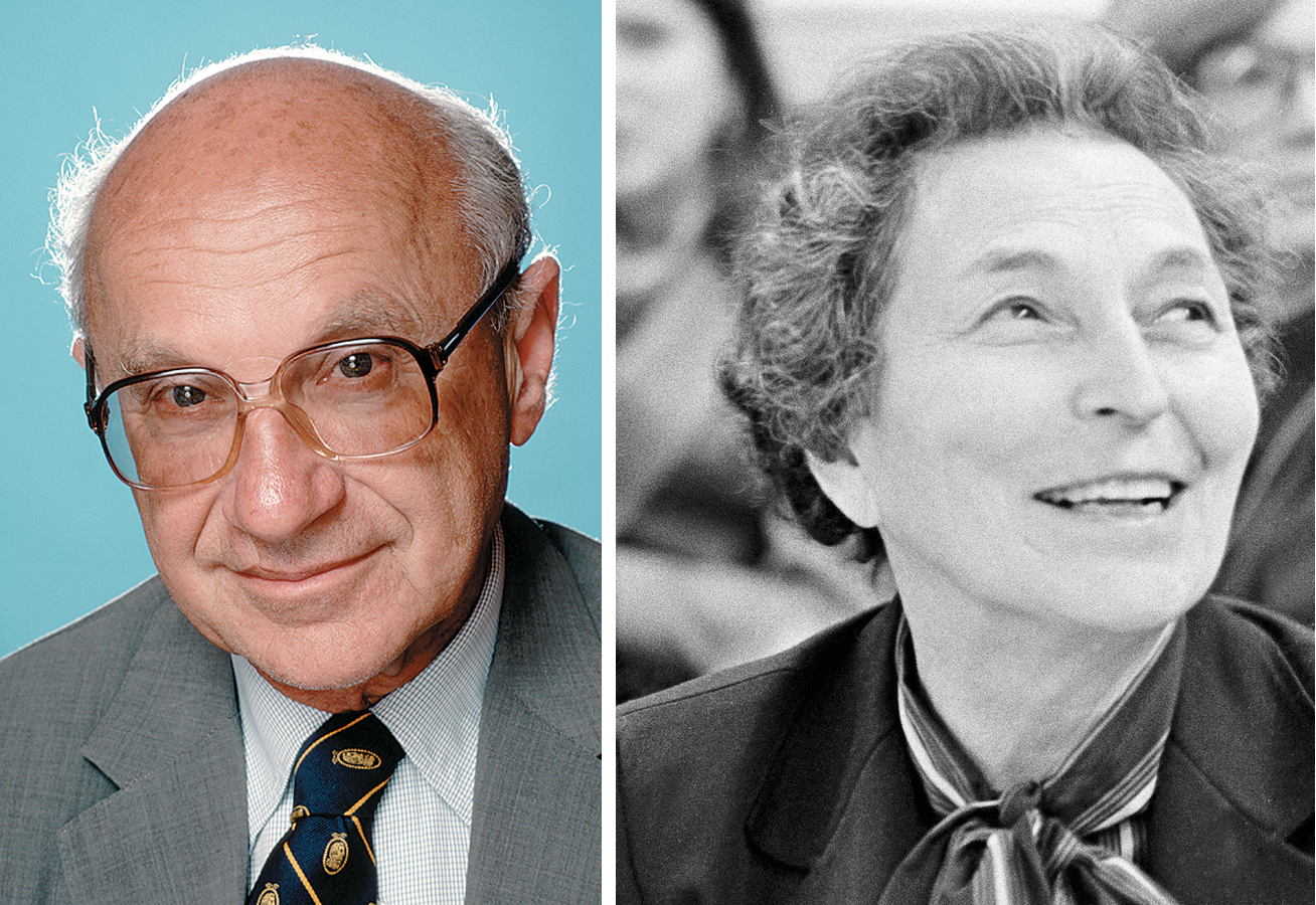
Teresa Zabala/The New York Times/Redux

Friedman and Schwartz showed that business cycles had historically been associated with fluctuations in the money supply. In particular, the money supply fell sharply during the onset of the Great Depression. Friedman and Schwartz persuaded many, though not all, economists that the Great Depression could have been avoided if the Federal Reserve had acted to prevent that monetary contraction and that monetary policy should play a key role in economic management.

The revival of interest in monetary policy was significant because it suggested that the burden of managing the economy could be shifted away from fiscal policy—meaning that economic management could largely be taken out of the hands of politicians. Fiscal policy, which must involve changing tax rates or government spending, necessarily involves political choices. If the government tries to stimulate the economy by cutting taxes, it must decide whose taxes will be cut. If it tries to stimulate the economy with government spending, it must decide what to spend the money on.

Monetary policy, in contrast, does not involve such choices: when the central bank cuts interest rates to fight a recession, it cuts everyone’s interest rate at the same time. So a shift from relying on fiscal policy to relying on monetary policy makes macroeconomics a more technical, less political issue. In fact, monetary policy in most major economies is set by an independent central bank that is insulated from the political process.

Monetarism

After the publication of A Monetary History, Milton Friedman led a movement, called monetarism, that sought to eliminate macroeconomic policy activism while maintaining the importance of monetary policy. Monetarism asserted that GDP will grow steadily if the money supply grows steadily. The monetarist policy prescription was to have the central bank target a constant rate of growth of the money supply, such as 3% per year, and maintain that target regardless of any fluctuations in the economy.

It’s important to realize that monetarism retained many Keynesian ideas. Like Keynes, Friedman asserted that the short run is important and that short-run changes in aggregate demand affect aggregate output as well as aggregate prices. Like Keynes, he argued that policy should have been much more expansionary during the Great Depression.

Monetarists argued, however, that most of the efforts of policy makers to smooth out the business cycle actually make things worse. We have already discussed concerns over the usefulness of discretionary fiscal policy—changes in taxes or government spending, or both—in response to the state of the economy. As we explained, government perceptions about the economy often lag behind reality, and there are further lags in changing fiscal policy and in its effects on the economy. As a result, discretionary fiscal policies intended to fight a recession often end up feeding a boom, and vice versa. According to monetarists, discretionary monetary policy, changes in the interest rate or the money supply by the central bank in order to stabilize the economy, faces the same problem of lags as fiscal policy, but to a lesser extent.

Friedman also argued that if the central bank followed his advice and refused to change the money supply in response to fluctuations in the economy, fiscal policy would be much less effective than Keynesians believed. Earlier we analyzed the phenomenon of crowding out, in which government deficits drive up interest rates and lead to reduced investment spending. Friedman and others pointed out that if the money supply is held fixed while the government pursues an expansionary fiscal policy, crowding out will limit the effect of the fiscal expansion on aggregate demand.

Figure 83-3 illustrates this argument. Panel (a) shows aggregate output and the aggregate price level. AD₁ is the initial aggregate demand curve and SRAS is the short-run aggregate supply curve. At the initial equilibrium, E₁, the level of aggregate output is Y₁ and the aggregate price level is P₁. Panel (b) shows the money market. MS is the money supply curve and MD₁ is the initial money demand curve, so the initial interest rate is r₁.

In panel (a) an expansionary fiscal policy shifts the AD curve rightward, driving up both the aggregate price level and aggregate output. However, this leads to an increase in the demand for money. If the money supply is held fixed, as in panel (b), the increase in money demand drives up the interest rate, reducing investment spending and offsetting part of the fiscal expansion. So the shift of the AD curve is less than it would otherwise be: fiscal policy becomes less effective when the money supply is held fixed.

Now suppose the government increases purchases of goods and services. We know that this will shift the AD curve rightward, as illustrated by the shift from AD₁ to AD₂; that aggregate output will rise, from Y₁ to Y₂; and that the aggregate price level will rise, from P₁ to P₂. Both the rise in aggregate output and the rise in the aggregate price level will, however, increase the demand for money, shifting the money demand curve rightward from MD₁ to MD₂. This drives up the equilibrium interest rate to r₂. Friedman’s point was that this rise in the interest rate reduces investment spending, partially offsetting the initial rise in government spending. As a result, the rightward shift of the AD curve is smaller than multiplier analysis indicates. And Friedman argued that with a constant money supply, the multiplier is so small that there’s not much point in using fiscal policy, even in a depressed economy.

But Friedman didn’t favor activist monetary policy either. He argued that the problem of time lags that limit the ability of discretionary fiscal policy to stabilize the economy also apply to discretionary monetary policy. Friedman’s solution was to put monetary policy on “autopilot.” The central bank, he argued, should follow a monetary policy rule, a formula that determines its actions and leaves it relatively little discretion. During the 1960s and 1970s, most monetarists favored a monetary policy rule of slow, steady growth in the money supply.

Underlying this view was the Quantity Theory of Money, which relies on the concept of the velocity of money, the ratio of nominal GDP to the money supply. Velocity is a measure of the number of times the average dollar bill in the economy turns over per year between buyers and sellers (e.g., I tip the Starbucks barista a dollar, she uses it to buy lunch, and so on). This concept gives rise to the velocity equation:

Where M is the money supply, V is velocity, P is the aggregate price level, and Y is real GDP.

Monetarists believed, with considerable historical justification, that the velocity of money was stable in the short run and changed only slowly in the long run. As a result, they claimed, steady growth in the money supply by the central bank would ensure steady growth in spending, and therefore in GDP.

Monetarism strongly influenced actual monetary policy in the late 1970s and early 1980s. It quickly became clear, however, that steady growth in the money supply didn’t ensure steady growth in the economy: the velocity of money wasn’t stable enough for such a simple policy rule to work.

Figure 83-4 shows how events eventually undermined the monetarists’ view. The figure shows the velocity of money, as measured by the ratio of nominal GDP to M1, from 1960 to 2013. As you can see, until 1980, velocity followed a fairly smooth, seemingly predictable trend. After the Fed began to adopt monetarist ideas in the late 1970s and early 1980s, however, the velocity of money began moving erratically—probably due to financial market innovations.

From 1960 to 1980, the velocity of money was stable, leading monetarists to believe that steady growth in the money supply would lead to a stable economy. After 1980, however, velocity began moving erratically, undermining the case for traditional monetarism. As a result, traditional monetarism fell out of favor.

Source: Bureau of Economic Analysis; Federal Reserve Bank of St. Louis.

Traditional monetarists are hard to find among today’s macroeconomists. As we’ll see later, however, the concern that originally motivated the monetarists—that too much discretionary monetary policy can actually destabilize the economy—has become widely accepted.

Inflation and the Natural Rate of Unemployment

At the same time that monetarists were challenging Keynesian views about how macroeconomic policy should be conducted, other economists—some, but not all, monetarists—were emphasizing the limits to what activist macroeconomic policy could achieve.

In the 1940s and 1950s, many Keynesian economists believed that expansionary fiscal policy could be used to achieve full employment on a permanent basis. In the 1960s, however, many economists realized that expansionary policies could cause problems with inflation, but they still believed policy makers could choose to trade off low unemployment for higher inflation even in the long run.

In 1968, however, Edmund Phelps of Columbia University and Milton Friedman, working independently, proposed the concept of the natural rate of unemployment. Earlier you learned that the natural rate of unemployment is also the nonaccelerating inflation rate of unemployment, or NAIRU. According to the natural rate hypothesis, because inflation is eventually embedded in expectations, to avoid accelerating inflation over time, the unemployment rate must be high enough that the actual inflation rate equals the expected rate of inflation. Attempts to keep the unemployment rate below the natural rate will lead to an ever-rising inflation rate.

The natural rate hypothesis limits the role of activist macroeconomic policy compared to earlier theories. Because the government can’t keep unemployment below the natural rate, its task is not to keep unemployment low but to keep it stable—to prevent large fluctuations in unemployment in either direction.

The Friedman–Phelps hypothesis made a strong prediction: that the apparent trade-off between unemployment and inflation would not survive an extended period of rising prices. Once inflation was embedded in the public’s expectations, inflation would continue even in the face of high unemployment. Sure enough, that’s exactly what happened in the 1970s. This accurate prediction was one of the triumphs of macroeconomic analysis, and it convinced the great majority of economists that the natural rate hypothesis was correct. In contrast to traditional monetarism, which declined in influence as more evidence accumulated, the natural rate hypothesis has become almost universally accepted among macroeconomists, with a few qualifications. But some macroeconomists believe that at very low or negative rates of inflation the hypothesis doesn’t work.

The Political Business Cycle

One final challenge to Keynesian economics focused not on the validity of the economic analysis but on its political consequences. A number of economists and political scientists pointed out that activist macroeconomic policy lends itself to political manipulation.

Shutterstock

Statistical evidence suggests that election results tend to be determined by the state of the economy in the months just before the election. In the United States, if the economy is growing rapidly and the unemployment rate is falling in the six months or so before Election Day, the incumbent party tends to be re-elected even if the economy performed poorly in the preceding three years.

AWesleyFloyd/Shutterstock

This creates an obvious temptation to abuse activist macroeconomic policy: pump up the economy in an election year, and pay the price in higher inflation and/or higher unemployment later. The result can be unnecessary instability in the economy, a political business cycle caused by the use of macroeconomic policy to serve political ends.

An often-cited example is the combination of expansionary fiscal and monetary policy that led to ra rapid growth in the U.S. economy just before the 1972 election and a sharp acceleration in inflation after the election. Kenneth Rogoff, a respected macroeconomist who served as chief economist at the International Monetary Fund, proclaimed Richard Nixon, the president at the time, “the all-time hero of political business cycles.”

One way to avoid a political business cycle is to place monetary policy in the hands of an independent central bank, insulated from political pressure. The political business cycle is also a reason to limit the use of discretionary fiscal policy to extreme circumstances.

Rational Expectations, Real Business Cycles, and New Classical Macroeconomics

As we have seen, one key difference between classical economics and Keynesian economics is that classical economists believed that the short-run aggregate supply curve is vertical, but Keynes emphasized the idea that the aggregate supply curve slopes upward in the short run. As a result, Keynes argued that demand shocks—shifts in the aggregate demand curve—can cause fluctuations in aggregate output.

The challenges to Keynesian economics that arose in the 1950s and 1960s—the renewed emphasis on monetary policy and the natural rate hypothesis—didn’t question the view that an increase in aggregate demand leads to a rise in aggregate output in the short run nor that a decrease in aggregate demand leads to a fall in aggregate output in the short run.

In the 1970s and 1980s, however, some economists developed an approach to the business cycle known as new classical macroeconomics, which returned to the classical view that shifts in the aggregate demand curve affect only the aggregate price level, not aggregate output. The new approach evolved in two steps. First, some economists challenged traditional arguments about the slope of the short-run aggregate supply curve based on the concept of rational expectations. Second, some economists suggested that changes in productivity caused economic fluctuations, a view known as real business cycle theory.

Rational Expectations

In the 1970s, a concept known as rational expectations had a powerful impact on macroeconomics. Rational expectations, a theory originally introduced by John Muth in 1961, is the view that individuals and firms make decisions optimally, using all available information.

For example, workers and employers bargaining over long-term wage contracts need to estimate the inflation rate they expect over the life of that contract. Rational expectations says that in making estimates of future inflation, they won’t just look at past rates of inflation; they will also take into account available information about monetary and fiscal policy. Suppose that prices didn’t rise last year, but that the monetary and fiscal policies announced by policy makers made it clear to economic analysts that there would be substantial inflation over the next few years. According to rational expectations, long-term wage contracts will be adjusted today to reflect this future inflation, even though prices didn’t rise in the past.

Rational expectations can significantly alter policy makers’ beliefs about the effectiveness of government policy. According to the original version of the natural rate hypothesis, a government attempt to trade off higher inflation for lower unemployment would work in the short run but would eventually fail because higher inflation would get built into expectations.

According to rational expectations, we should remove the word eventually: if it’s clear that the government intends to trade off higher inflation for lower unemployment, the public will understand this, and expected inflation will immediately rise. So, under rational expectations, government intervention fails in the short run and the long run.

In the 1970s, Robert Lucas of the University of Chicago used this logic to argue that monetary policy can change the level of unemployment only if it comes as a surprise to the public. If his analysis was right, monetary policy isn’t useful in stabilizing the economy after all. In 1995 Lucas won the Nobel Prize in economics for this work, which remains widely admired. However, many—perhaps most—macroeconomists, especially those advising policy makers, now believe that his conclusions were overstated.

Why, in the view of many macroeconomists, doesn’t the rational expectations hypothesis accurately describe how the economy behaves? New Keynesian economics, a set of ideas that became influential in the 1990s, provides an explanation. It argues that market imperfections interact to make many prices in the economy temporarily sticky. For example, one new Keynesian argument points out that monopolists don’t have to be too careful about setting prices exactly “right”: if they set a price a bit too high, they’ll lose some sales but make more profit on each sale; if they set the price too low, they’ll reduce the profit per sale but sell more. As a result, even small costs to changing prices can lead to substantial price stickiness and make the economy as a whole behave in a Keynesian fashion.

Over time, new Keynesian ideas combined with actual experience have reduced the practical influence of the rational expectations concept. Nonetheless, the idea of rational expectations served as a useful caution for macroeconomists who had become excessively optimistic about their ability to manage the economy.

Real Business Cycles

Earlier we introduced the concept of total factor productivity, the amount of output that can be generated with a given level of factor inputs. Total factor productivity grows over time, but that growth isn’t smooth. In the 1980s, a number of economists argued that slowdowns in productivity growth, which they attributed to pauses in technological progress, are the main cause of recessions. Real business cycle theory claims that fluctuations in the rate of growth of total factor productivity cause the business cycle.

Believing that the aggregate supply curve is vertical, real business cycle theorists attribute the source of business cycles to shifts of the aggregate supply curve: a recession occurs when a slowdown in productivity growth shifts the aggregate supply curve leftward, and a recovery occurs when a pickup in productivity growth shifts the aggregate supply curve rightward. In the early days of real business cycle theory, the theory’s proponents denied that changes in aggregate demand—and likewise, macroeconomic policy activism—had any effect on aggregate output.

This theory was strongly influential, but the current status of real business cycle theory is somewhat similar to that of rational expectations. The theory is widely recognized as having made valuable contributions to our understanding of the economy, and it serves as a useful caution against too much emphasis on aggregate demand.

But many of the real business cycle theorists themselves now acknowledge that their models need an upward-sloping aggregate supply curve to fit the economic data—and that this gives aggregate demand a potential role in determining aggregate output. And as we have seen, policy makers strongly believe that aggregate demand policy has an important role to play in fighting recessions.

Module 83 Review

Check Your Understanding

For each of the following economic theories, identify its fundamental conclusion.

• a. the classical model of the price level
• b. Keynesian economics
• c. monetarism
• d. the natural rate hypothesis
• e. rational expectations
• f. real business cycle theory