Calculating GDP
We’ve just explained that there are in fact three methods for calculating GDP:
adding up total value of all final goods and services produced
adding up spending on all domestically produced goods and services
adding up total factor income earned by households from firms in the economy
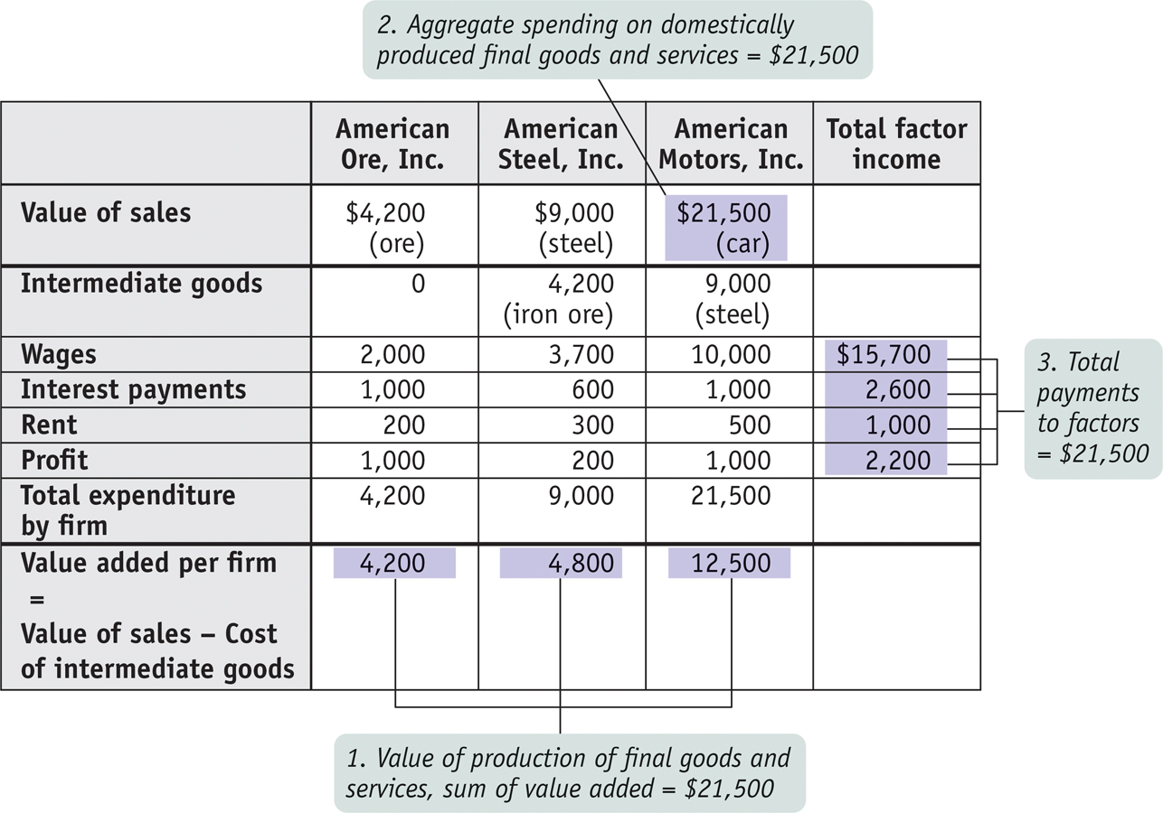
Government statisticians use all three methods. To illustrate how these three methods work, we will consider a hypothetical economy, shown in Figure 7-2. This economy consists of three firms—
Measuring GDP as the Value of Production of Final Goods and Services The first method for calculating GDP is to add up the value of all the final goods and services produced in the economy—
To understand why only final goods and services are included in GDP, look at the simplified economy described in Figure 7-2. Should we measure the GDP of this economy by adding up the total sales of the iron ore producer, the steel producer, and the auto producer? If we did, we would in effect be counting the value of the steel twice—
The value added of a producer is the value of its sales minus the value of its purchases of intermediate goods and services.
So counting the full value of each producer’s sales would cause us to count the same items several times and artificially inflate the calculation of GDP. For example, in Figure 7-2, the total value of all sales, intermediate and final, is $34,700: $21,500 from the sale of the car, plus $9,000 from the sale of the steel, plus $4,200 from the sale of the iron ore. Yet we know that GDP is only $21,500. The way we avoid double-
That is, we subtract the cost of inputs—

Measuring GDP as Spending on Domestically Produced Final Goods and Services Another way to calculate GDP is by adding up aggregate spending on domestically produced final goods and services. That is, GDP can be measured by the flow of funds into firms. Like the method that estimates GDP as the value of domestic production of final goods and services, this measurement must be carried out in a way that avoids double-
In terms of our steel and auto example, we don’t want to count both consumer spending on a car (represented in Figure 7-2 by $12,500, the sales price of the car) and the auto producer’s spending on steel (represented in Figure 7-2 by $9,000, the price of a car’s worth of steel). If we counted both, we would be counting the steel embodied in the car twice. We solve this problem by counting only the value of sales to final buyers, such as consumers, firms that purchase investment goods, the government, or foreign buyers. In other words, in order to avoid double-
FOR INQUIRING MINDS: Our Imputed Lives

An old line says that when a person marries the household cook, GDP falls. And it’s true: when someone provides services for pay, those services are counted as a part of GDP. But the services family members provide to each other are not. Some economists have produced alternative measures that try to “impute” the value of household work—
GDP estimates do, however, include an imputation for the value of “owner-
If you think about it, this makes a lot of sense. In a home-
As we’ve already pointed out, the national accounts do include investment spending by firms as a part of final spending. That is, an auto company’s purchase of steel to make a car isn’t considered a part of final spending, but the company’s purchase of new machinery for its factory is considered a part of final spending. What’s the difference? Steel is an input that is used up in production; machinery will last for a number of years. Since purchases of capital goods that will last for a considerable time aren’t closely tied to current production, the national accounts consider such purchases a form of final sales.
In later chapters, we will make use of the proposition that GDP is equal to aggregate spending on domestically produced goods and services by final buyers. We will also develop models of how final buyers decide how much to spend. With that in mind, we’ll now examine the types of spending that make up GDP.
Look again at the markets for goods and services in Figure 7-1, and you will see that one component of sales by firms is consumer spending. Let’s denote consumer spending with the symbol C. Figure 7-1 also shows three other components of sales: sales of investment goods to other businesses, or investment spending, which we will denote by I; government purchases of goods and services, which we will denote by G; and sales to foreigners—
In reality, not all of this final spending goes toward domestically produced goods and services. We must take account of spending on imports, which we will denote by IM. Income spent on imports is income not spent on domestic goods and services—

We’ll be seeing a lot of Equation 7-
PITFALLS: GDP: WHAT’S IN AND WHAT’S OUT
GDP: WHAT’S IN AND WHAT’S OUT
It’s easy to confuse what is included in and what is excluded from GDP. So let’s stop here for a moment and make sure the distinction is clear. The most likely source of confusion is the difference between investment spending and spending on intermediate goods and services. Investment spending—
Why the difference? Recall from Chapter 2 that we made a distinction between resources that are used up and those that are not used up in production. An input, like steel, is used up in production. An investment good, like a metal-
Spending on changes to inventories is considered a part of investment spending, so it is also included in GDP. Why? Because, like a machine, additional inventory is an investment in future sales. And when a good is released for sale from inventories, its value is subtracted from the value of inventories and so from GDP.
Used goods are not included in GDP because, as with inputs, to include them would be to double-
Also, financial assets such as stocks and bonds are not included in GDP because they don’t represent either the production or the sale of final goods and services. Rather, a bond represents a promise to repay with interest, and a stock represents a proof of ownership. And for obvious reasons, foreign-
Here is a summary of what’s included and not included in GDP:
Included
Domestically produced final goods and services, including capital goods, new construction of structures, and changes to inventories
Not Included
Intermediate goods and services
Inputs
Used goods
Financial assets like stocks and bonds
Foreign-
produced goods and services
Measuring GDP as Factor Income Earned from Firms in the Economy A final way to calculate GDP is to add up all the income earned by factors of production from firms in the economy—
Figure 7-2 shows how this calculation works for our simplified economy. The numbers shaded in the column at far right show the total wages, interest, and rent paid by all these firms as well as their total profit. Summing up all of these items yields total factor income of $21,500—
We won’t emphasize factor income as much as the other two methods of calculating GDP. It’s important to keep in mind, however, that all the money spent on domestically produced goods and services generates factor income to households—
The Components of GDP Now that we know how GDP is calculated in principle, let’s see what it looks like in practice.
Figure 7-3 shows the first two methods of calculating GDP side by side. The height of each bar above the horizontal axis represents the GDP of the U.S. economy in 2013: $16,800 billion. Each bar is divided to show the breakdown of that total in terms of where the value was added and how the money was spent.
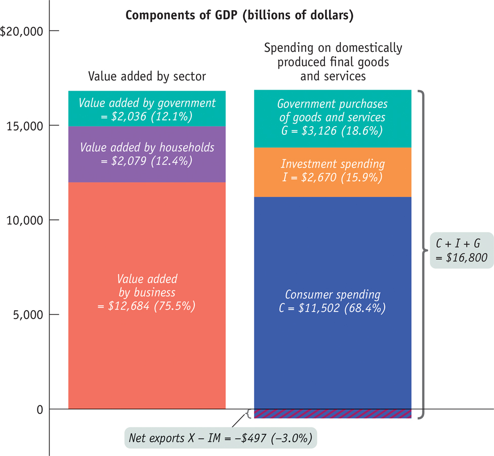
In the left bar in Figure 7-3, we see the breakdown of GDP by value added according to sector, the first method of calculating GDP. Of the $16,800 billion, $12,684 billion consisted of value added by businesses. Another $2,079 billion of value added was added by households and institutions; a large part of that was the imputed services of owner-
The right bar in Figure 7-3 corresponds to the second method of calculating GDP, showing the breakdown by the four types of aggregate spending. The total length of the right bar is longer than the total length of the left bar, a difference of $497 billion (which, as you can see, is the amount by which the right bar extends below the horizontal axis). That’s because the total length of the right bar represents total spending in the economy, spending on both domestically produced and foreign-
Net exports are the difference between the value of exports and the value of imports.
But some of that spending was absorbed by foreign-
!worldview! FOR INQUIRING MINDS: Gross What?
Occasionally you may see references not to gross domestic product but to gross national product, or GNP. Is this just another name for the same thing? Not quite.
If you look at Figure 7-1 carefully, you may realize that there’s a possibility that is missing from the figure. According to the figure, all factor income goes to domestic households. But what happens when profits are paid to foreigners who own stock in General Motors or Apple? And where do the profits earned by American companies operating overseas fit in?
To answer these questions, an alternative measure, GNP, was devised. GNP is defined as the total factor income earned by residents of a country. It excludes factor income earned by foreigners, like profits paid to foreign investors who own American stocks and payments to foreigners who work temporarily in the United States. And it includes factor income earned abroad by Americans, like the profits of Apple’s European operations that accrue to Apple’s American shareholders and the wages of Americans who work abroad temporarily.

In the early days of national income accounting, economists usually used GNP rather than GDP as a measure of the economy’s size—
In practice, it doesn’t make much difference which measure is used for large economies like that of the United States, where the flows of net factor income to other countries are relatively small. In 2013, America’s GNP was about 1.5% larger than its GDP, mainly because of the overseas profit of U.S. companies. However, for smaller countries, which are likely to be hosts to a number of foreign companies, GDP and GNP can diverge significantly. For example, much of Ireland’s industry is owned by American corporations, whose profit must be deducted from Ireland’s GNP. In addition, Ireland has become a host to many temporary workers from poorer regions of Europe, whose wages must also be deducted from Ireland’s GNP. As a result, in 2013 Ireland’s GNP was only 86% of its GDP.