1.2 Module 41: The Phillips Curve

WHAT YOU WILL LEARN
 What the Phillips curve is and the nature of the short-
run trade- off between inflation and unemployment  Why there is no long-
run trade- off between inflation and unemployment  Why expansionary policies are limited due to the effects of expected inflation
 Why deflation is a problem for economic policy
Inflation and Unemployment in the Short Run
We’ve just seen that expansionary policies lead to a lower unemployment rate. Our next step in understanding the temptations and dilemmas facing governments is to show that there is a short-
The Short-Run Phillips Curve
The origins of this concept lie in a famous 1958 paper by the New Zealand–
Looking at evidence like Figure 41-1, many economists concluded that there is a negative short-


The short-
Early estimates of the short-
Even at the time, however, some economists argued that a more accurate short-
In general, a negative supply shock shifts SRPC up, as the inflation rate increases for every level of the unemployment rate, and a positive supply shock shifts it down as the inflation rate falls for every level of the unemployment rate. Both outcomes are shown in Figure 41-3.

But supply shocks are not the only factors that can change the inflation rate. In the early 1960s, Americans had little experience with inflation as inflation rates had been low for decades. But by the late 1960s, after inflation had been steadily increasing for a number of years, Americans had come to expect future inflation. In 1968 two economists—
Inflation Expectations and the Short-Run Phillips Curve
The expected rate of inflation is the rate that employers and workers expect in the near future. One of the crucial discoveries of modern macroeconomics is that changes in the expected rate of inflation affect the short-
Why do changes in expected inflation affect the short-
For these reasons, an increase in expected inflation shifts the short-
Figure 41-4 shows how the expected rate of inflation affects the short-

Alternatively, suppose the expected rate of inflation is 2%. In that case, employers and workers will build this expectation into wages and prices: at any given unemployment rate, the actual inflation rate will be 2 percentage points higher than it would be if people expected 0% inflation. SRPC2, which shows the Phillips curve when the expected inflation rate is 2%, is SRPC0 shifted upward by 2 percentage points at every level of unemployment. According to SRPC2, the actual inflation rate will be 2% if the unemployment rate is 6%; it will be 4% if the unemployment rate is 4%.
What determines the expected rate of inflation? In general, people base their expectations about inflation on experience. If the inflation rate has hovered around 0% in the last few years, people will expect it to be around 0% in the near future. But if the inflation rate has averaged around 5% lately, people will expect inflation to be around 5% in the near future.
Since expected inflation is an important part of the modern discussion about the short-
Inflation and Unemployment in the Long Run
The short-
However, this view was greatly altered by the later recognition that expected inflation affects the short-
So what does the trade-
The Long-Run Phillips Curve
Figure 41-5 reproduces the two short-
Suppose that the economy has, in the past, had a 0% inflation rate. In that case, the current short-
Also suppose that policy makers decide to trade off lower unemployment for a higher rate of inflation. They use monetary policy, fiscal policy, or both to drive the unemployment rate down to 4%. This puts the economy at point A on SRPC0, leading to an actual inflation rate of 2%.
Over time, the public will come to expect a 2% inflation rate. This increase in inflationary expectations will shift the short-
Eventually, the 4% actual inflation rate gets built into expectations about the future inflation rate, and the short-
To avoid accelerating inflation over time, the unemployment rate must be high enough that the actual rate of inflation matches the expected rate of inflation. This is the situation at E0 on SRPC0: when the expected inflation rate is 0% and the unemployment rate is 6%, the actual inflation rate is 0%. It is also the situation at E2 on SRPC2: when the expected inflation rate is 2% and the unemployment rate is 6%, the actual inflation rate is 2%. And it is the situation at E4 on SRPC4: when the expected inflation rate is 4% and the unemployment rate is 6%, the actual inflation rate is 4%. As we’ll learn shortly, this relationship between accelerating inflation and the unemployment rate is known as the natural rate hypothesis.
The unemployment rate at which inflation does not change over time—

The nonaccelerating inflation rate of unemployment, or NAIRU, is the unemployment rate at which inflation does not change over time.
The long-
We can now explain the significance of the vertical line LRPC. It is the long-
The Natural Rate of Unemployment, Revisited
Recall the concept of the natural rate of unemployment, the portion of the unemployment rate unaffected by the swings of the business cycle. Now we have introduced the concept of the NAIRU. How do these two concepts relate to each other?
The answer is that the NAIRU is another name for the natural rate. The level of unemployment the economy “needs” in order to avoid accelerating inflation is equal to the natural rate of unemployment.
In fact, economists estimate the natural rate of unemployment by looking for evidence about the NAIRU from the behavior of the inflation rate and the unemployment rate over the course of the business cycle. For example, the way major European countries learned, to their dismay, that their natural rates of unemployment were 9% or more was through unpleasant experience. In the late 1980s, and again in the late 1990s, European inflation began to accelerate as European unemployment rates, which had been above 9%, began to fall, approaching 8%.
THE GREAT DISINFLATION OF THE 1980s
As we’ve mentioned several times, the United States ended the 1970s with a high rate of inflation, at least by its own peacetime historical standards—
By the mid-

How was this disinflation achieved? At great cost. Beginning in late 1979, the Federal Reserve imposed strongly contractionary monetary policies, which pushed the economy into its worst recession since the Great Depression. Panel (b) shows the Congressional Budget Office estimate of the U.S. output gap from 1979 to 1989: by 1982, actual output was 7% below potential output, corresponding to an unemployment rate of more than 9%. Aggregate output didn’t get back to potential output until 1987.
Our analysis of the Phillips curve tells us that a temporary rise in unemployment, like that of the 1980s, is needed to break the cycle of inflationary expectations. Once expectations of inflation are reduced, the economy can return to the natural rate of unemployment at a lower inflation rate. And that’s just what happened.
But the cost was huge. If you add up the output gaps over 1980–
In Figure 41-3 we cited Congressional Budget Office estimates of the U.S. natural rate of unemployment. The CBO has a model that predicts changes in the inflation rate based on the deviation of the actual unemployment rate from the natural rate. Given data on actual unemployment and inflation, this model can be used to deduce estimates of the natural rate—
The Costs of Disinflation
Through experience, policy makers have found that bringing inflation down is a much harder task than increasing it. The reason is that once the public has come to expect continuing inflation, bringing inflation down is painful.
A persistent attempt to keep unemployment below the natural rate leads to accelerating inflation that becomes incorporated into expectations. To reduce inflationary expectations, policy makers need to run the process in reverse, adopting contractionary policies that keep the unemployment rate above the natural rate for an extended period of time. The process of bringing down inflation that has become embedded in expectations is known as disinflation.
Disinflation can be very expensive. The U.S. retreat from high inflation at the beginning of the 1980s appears to have cost the equivalent of about 18% of a year’s real GDP, the equivalent of roughly $2.6 trillion today. The justification for paying these costs is that they lead to a permanent gain. Although the economy does not recover the short-
Some economists argue that the costs of disinflation can be reduced if policy makers explicitly state their determination to reduce inflation. A clearly announced, credible policy of disinflation, they contend, can reduce expectations of future inflation and so shift the short-
Deflation
Before World War II, deflation—a falling aggregate price level—
Why is deflation a problem? And why is it hard to end?
Debt Deflation
Deflation, like inflation, produces both winners and losers—

Debt deflation is the reduction in aggregate demand arising from the increase in the real burden of outstanding debt caused by deflation.
In a famous analysis at the beginning of the Great Depression, economist Irving Fisher claimed that the effects of deflation on borrowers and lenders can worsen an economic slump. Deflation, in effect, takes real resources away from borrowers and redistributes them to lenders. Fisher argued that borrowers, who lose from deflation, are typically short of cash and will be forced to cut their spending sharply when their debt burden rises. Lenders, however, are less likely to increase spending sharply when the values of the loans they own rise. The overall effect, said Fisher, is that deflation reduces aggregate demand, deepening an economic slump, which, in a vicious circle, may lead to further deflation. The effect of deflation in reducing aggregate demand, known as debt deflation, probably played a significant role in the Great Depression.
Effects of Expected Deflation
Like expected inflation, expected deflation affects the nominal interest rate. Consider Figure 41-7 (which you may recall seeing in an earlier section). It demonstrates how expected inflation affects the equilibrium interest rate. As shown, the equilibrium nominal interest rate is 4% if the expected inflation rate is 0%. Clearly, if the expected inflation rate is −3%—if the public expects deflation at 3% per year—

D0 and S0 are the demand and supply curves for loanable funds when the expected future inflation rate is 0%. At an expected inflation rate of 0%, the equilibrium nominal interest rate is 4%. An increase in expected future inflation pushes both the demand and supply curves upward by 1 percentage point for every percentage point increase in expected future inflation. D10 and S10 are the demand and supply curves for loanable funds when the expected future inflation rate is 10%. The 10 percentage point increase in expected future inflation raises the equilibrium nominal interest rate to 14%. The expected real interest rate remains at 4%, and the equilibrium quantity of loanable funds also remains unchanged.
There is a zero bound on the nominal interest rate: it cannot go below zero.
But what would happen if the expected rate of inflation were −5%? Would the nominal interest rate fall to −1%, meaning that lenders are paying borrowers 1% on their debt? No. Nobody would lend money at a negative nominal rate of interest because they could do better by simply holding cash. This illustrates what economists call the zero bound on the nominal interest rate: it cannot go below zero.
This zero bound can limit the effectiveness of monetary policy. Suppose the economy is depressed, with output below potential output and the unemployment rate above the natural rate. Normally, the central bank can respond by cutting interest rates so as to increase aggregate demand. If the nominal interest rate is already zero, however, the central bank cannot push it down any further. Banks refuse to lend and consumers and firms refuse to spend because, with a negative inflation rate and a 0% nominal interest rate, holding cash yields a positive real rate of return. Any further increases in the monetary base will either be held in bank vaults or held as cash by individuals and firms, without being spent.
A liquidity trap is a situation in which conventional monetary policy is ineffective because nominal interest rates are up against the zero bound.
A situation in which conventional monetary policy to fight a slump—

However, the recent history of the Japanese economy, shown in Figure 41-9, provides a modern illustration of the problem of deflation and the liquidity trap. Japan experienced a huge boom in the prices of both stocks and real estate in the late 1980s, and then saw both bubbles burst. The result was a prolonged period of economic stagnation, the so-


In an effort to fight the weakness of the economy, the Bank of Japan—
In the aftermath of the 2008 financial crisis, the Federal Reserve also found itself up against the zero bound with the interest on short-
!world_eia!THE DEFLATION SCARE OF 2010
Ever since the financial crisis of 2008, U.S. policy makers have been worried about the possibility of “Japanification”—that is, they have worried that, like Japan since the 1990s, the United States might find itself stuck in a deflationary trap. Indeed, Ben Bernanke, chairman of the Federal Reserve during the crisis, studied Japan intensively before he went to the Fed and sought to do better than his Japanese counterparts.
Fears of deflation were particularly intense in the summer and early fall of 2010. Figure 41-10 shows why, by tracking two numbers the Fed watches carefully when making policy. One of these numbers is the “core” inflation rate over the past year—

As you can see, by the late summer of 2010 both actual inflation and expected inflation were sliding to levels well below the Fed’s 2% target. Fed officials were worried, and they took action. In August 2010 Bernanke gave a speech at the annual Fed meeting, signaling that he would take special actions to head off the deflationary threat. And in November the Fed, which normally buys only short-
The figure shows that Bernanke’s speech and the Fed’s action led to a major change in expectations, as investors’ fears of deflation ebbed. Actual inflation also picked up significantly.
What was far from clear, however, was whether the Fed had achieved more than a temporary reprieve. A year after Bernanke’s big speech, expected inflation was sagging again, and deflation fears were on the rise. And those fears linger, given that core inflation averaged only 1.8% in 2013.
Module 41 Review
Solutions appear at the back of the book.
Check Your Understanding
Explain how the short-
run Phillips curve illustrates the negative relationship between cyclical unemployment and the actual inflation rate for a given level of the expected inflation rate. Why is there no long-
run trade- off between unemployment and inflation? Why is disinflation so costly for an economy? Are there ways to reduce these costs?
Why won’t anyone lend money at a negative nominal rate of interest? How can this pose problems for monetary policy?
Multiple-
Question
it7d0MQfBD/0fHRLWV/uV5R1q0/K/6KPElwI4gwKCg8m7draJHM7i81wpvZYi0LX90seF4WwB/ibo1+UexCng0ccaD/I3L/nIl76vQRs4UuSYTtJk50W5UzlDz/vKf+4Cp6o45/MqoqEXu6Z9rfjL54ryMU0H/7xU5uXn/B2QdT3N5uciOU9/hL7Rx7WjRO5OMxNGsKDZBYLChyYTshvsiEFYNgmEUn3J1fyUyWZkIU+BIODdZ/xO0/u50myqiuJAiL8iKHAeIDybpU/LdE8I4l+juVDpjt1raHaONvOHN6PEsSAT6kbofReNNfTpkRpkoaf6IXhIz9WTZDuX9MHBCMQBjr9qyZ+kiZzMV9A0Uk+K+tV+5pN2Hpc6Mbjhs1lQzkXHVSwIjEzR2K7rY7yJXSghaZI1OHe1wgQ6KzbLIv4K670d5d0N+wbRo7Z70STH4MAjMkSPxQvEQkfCOA6NUkgRqHxTM6YYi7axQof+vAntEH39jR7IhlzvlKkIS36GUjkIzoRYnvVz08abFyMmg6eu/ZoopRiPljC30ezT6Y5ZSbj8+HCnMW+SJp7xVOtfFeLwaGuFPg57p3T5Y8j3xproZ0=Question
HZlMaTmTuz2cAfGxuy+G5LlySUye5QAymbd2fQqwqghNWEfifjKUyZtAgJoE3Gsw8jZBw5nc3zkuW1Oi3g9jJL4Isvta+pPvG0LO+wmF5yzFPhoe6j71IoCMtsPnkXlPGeK/DZVS3CdobalOQhpzV+3i8W+M35PJyV3N2PdSo9FyuDaOu31Gu/PAJs2nS4ANni1w88D8QK3o1Dwzgmm6HplRlYRzVOLtzLiBMf3A1sZg8d5sXjw1QPiPyUWx53CeXmuddLn6Wf5F5Jtcd/wb81PNLrDEE6ok4oJRAJ2+Bsh3BwCG5w1cica6mUkUlEmAY/DKsoSuAcEhr7UC1ikoIvvraqiwAWurCGYyQ3VENivnU+70jDTVhoUGj2RjSkGbskuLaBZuaihDdX+EFbO44raZhl3wWrDdrLHERfywAKZUeaH2s3i7SS66XzJihgUn/7s9aO6gXpAdlysXQKQsw0nx0rG2eU1VCpw8F8wIue1MmbS6xQI7ZsbkC7hjUYpoUuCtfu11cco06zZxmqOg54bBX3KI/7WY3OJcVnpfspMYiVEO+GbA3g==Question
NS1p8eR445JA0cGEfPH0Tq/UK7qD1HqvQpSITFeGjbB7rPLYXxDWO/iPy6EZmDMtrRdAZUXgeiofP6cVTeJcsUCxMdisHjv7+M8qaq5J5fB/Gm+0NXHrqbw2FGIRJBDfZhJYdtE63Ss6T2ckEzhf3CR15SOn22sl+wwpAoHtCZN6FYMbRK7IoGt8RdWoOwPadOTkfzz2ot5rd+9rNyX8+T4MjnostFTSiFHlLLkRcYC2lr5zof7xF1eRPjuyCXfSsvvfbIgEwuAOZ7f3TFbE/QCCaklrkahKPIOAVyOKCzzY7doFvTe5lfFXrbu71cPh483JgUeFc8ZGPPfN1S0/nQfYjlSWTnAPeVofk/u5si7PwuzV+Bu15dkUy2pxL4Ds3szB7LbMnALz5wYsAw66iU6BjLjMvMkQQ+bh3D1EkbvEZzRdE0YNrpVaMN5VUHo8z09belVHRvU3ss7drzOvKGPTkMNpi9A9tA9nvXqpBOTlEepb0NEoSJkfueY/pu+ydtqY5UQziqosz0XgLD32ljfhTwRON5Ue2e5NhNV7092/BArXffm0A979Pf74lcEyy988HmMeO1Kol9gygEvl1i2SNXVutJLvHODdpArAYj92/yECcYhNRYE2CbOmpzdEqN4+StnpudTFpYCNZJPx6DKm83Ne8DW5ANwmdVuF8tKrK7t75pG8zy+R6XBTIBgQtppKv/5lAA6c8kuGuV8kwS/vM4y26nnw3KKBmwCmSrea11VUIZTZn8s0DEy72PTpIRT8Dg==Question
mIf+7srI8Luz7Jznq5G/azSxYNHn9iLCqjOkMxwR3hSftKcvl+rpVjYFuziiryEuLoJPN1f5AvCi1eztnfy0TdexWtts3TeBdzBq2qoYVrIkM+nHg2otcDbPVlVHmm0BY6E3OGycJY77l2xuamNZ6ZP0B2BnM1hARb3TlGqOTf8bp6CB1WFNjMX9/2L70UyI8hC4gTaeUqCKTtCjNT8rZcybpfB+t5wMqGA6/4rvopC9HBRdFwJ+yuKEc4D8dYsxkhqfdnqlGDjiCFrV5PwY+vPjsLgaWhbJmJWRZ3lo9zK51rmqPLWfyiF0JoS+CFRkeFm7ChOA3YXc5h/3Question
LzVnPVX+JBJTtpqBChgAz9sSSUbH99KqxDxJhXmamtQkx4zoDcsfhJFQSelVvE0Prf+32BStumQpwGz1GI5KNR0Md+3rTIKgzem1wAp3gO3jFWdrg8iuufMbcC+nMQdL8rnHsVpdSiRwqoKmBvWPsYDRt7YT5nFeWUXt3RJnDMuq/IKPIjiETCfexwRblcHWZLuyBKF5ZQN0aacvQ9NctxSZSOB3o2sILvkca5yZQV2OQ5XOqGSqRIawbS9guS/OoxbdTxDmE7zMEvv6RJHPR05IxdRgZv3EBmMpyY/gONTMXgbIPHBLRXqUAlotDGO5ynE98bjhA4C9smZVArXGf5qAMHk/MCjLVqEaLQIitCNPr7Kp1voI1w5KB6UzCZOzAz6Hi0DEcjrKl+E4PqWIwjjyLD4=
Critical-
Use the accompanying diagram to answer the questions that follow.
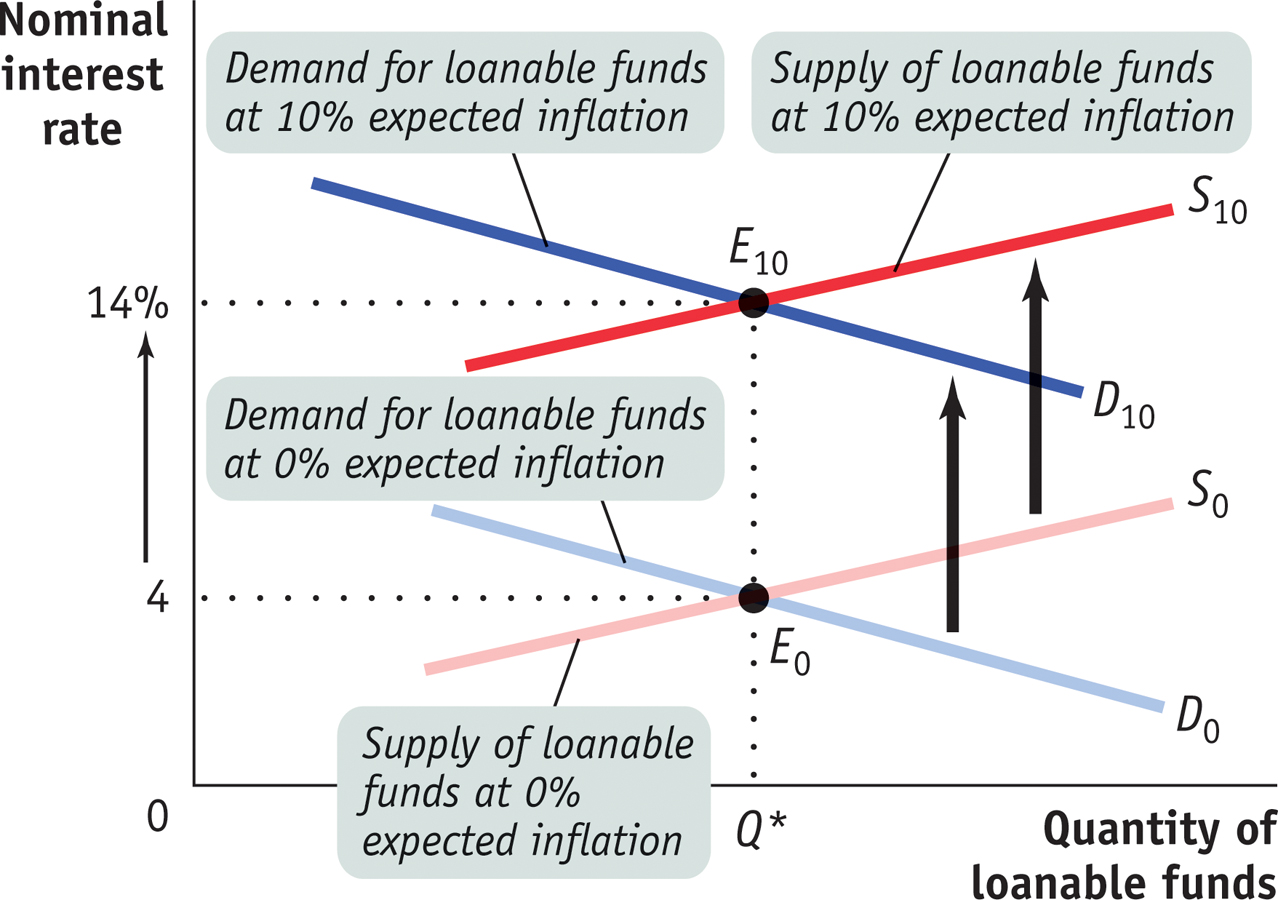
What is the nominal interest rate if expected inflation is 0%?
What would the nominal interest rate be if the expected inflation rate were −2%? Explain.
What would the nominal interest rate be if the expected inflation rate were −6%? Explain.
What would a negative nominal interest rate mean for lenders? How much lending would take place at a negative nominal interest rate? Explain.
What effect does a nominal interest rate of zero have on monetary policy? What is this situation called?