Income–Expenditure Equilibrium
For all but one value of real GDP shown in Table 11-2, real GDP is either more or less than AEPlanned, the sum of consumer spending and planned investment spending. For example, when real GDP is 1,000, consumer spending, C, is 900 and planned investment spending is 500, making planned aggregate spending 1,400. This is 400 more than the corresponding level of real GDP. Now consider what happens when real GDP is 2,500; consumer spending, C, is 1,800 and planned investment spending is 500, making planned aggregate spending only 2,300, 200 less than real GDP.
As we’ve just explained, planned aggregate spending can be different from real GDP only if there is unplanned inventory investment, IUnplanned, in the economy. Let’s examine Table 11-3, which includes the numbers for real GDP and for planned aggregate spending from Table 11-2. It also includes the levels of unplanned inventory investment, IUnplanned, that each combination of real GDP and planned aggregate spending implies. For example, if real GDP is 2,500, planned aggregate spending is only 2,300. This 200 excess of real GDP over AEPlanned must consist of positive unplanned inventory investment. This can happen only if firms have overestimated sales and produced too much, leading to unintended additions to inventories. More generally, any level of real GDP in excess of 2,000 corresponds to a situation in which firms are producing more than consumers and other firms want to purchase, creating an unintended increase in inventories.
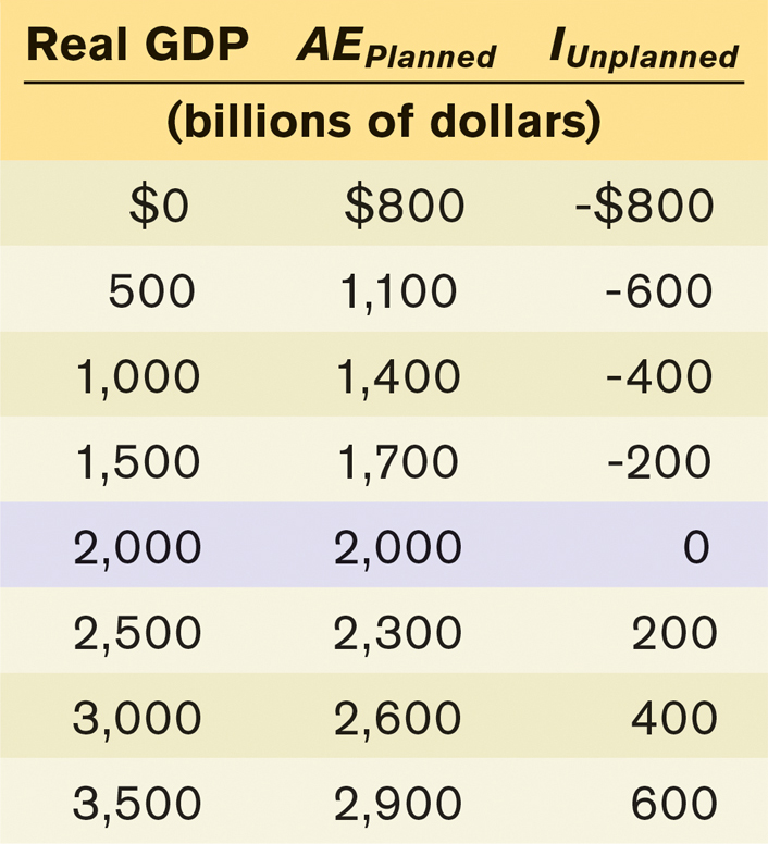
TABLE 11-3
Conversely, a level of real GDP below 2,000 implies that planned aggregate spending is greater than real GDP. For example, when real GDP is 1,000, planned aggregate spending is much larger, at 1,400. The 400 excess of AEPlanned over real GDP corresponds to negative unplanned inventory investment equal to −400. More generally, any level of real GDP below 2,000 implies that firms have underestimated sales, leading to a negative level of unplanned inventory investment in the economy.
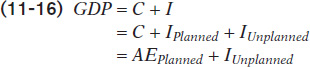
By putting together Equations 11-10, 11-11, and 11-14, we can summarize the general relationships among real GDP, planned aggregate spending, and unplanned inventory investment as follows:
So whenever real GDP exceeds AEPlanned, IUnplanned is positive; whenever real GDP is less than AEPlanned, IUnplanned is negative.
But firms will act to correct their mistakes. We’ve assumed that they don’t change their prices, but they can adjust their output. Specifically, they will reduce production if they have experienced an unintended rise in inventories or increase production if they have experienced an unintended fall in inventories. And these responses will eventually eliminate the unanticipated changes in inventories and move the economy to a point at which real GDP is equal to planned aggregate spending.
Staying with our example, if real GDP is 1,000, negative unplanned inventory investment will lead firms to increase production, leading to a rise in real GDP. In fact, this will happen whenever real GDP is less than 2,000—that is, whenever real GDP is less than planned aggregate spending. Conversely, if real GDP is 2,500, positive unplanned inventory investment will lead firms to reduce production, leading to a fall in real GDP. This will happen whenever real GDP is greater than planned aggregate spending.
The economy is in income–expenditure equilibrium when aggregate output, measured by real GDP, is equal to planned aggregate spending.
The only situation in which firms won’t have an incentive to change output in the next period is when aggregate output, measured by real GDP, is equal to planned aggregate spending in the current period, an outcome known as income–expenditure equilibrium. In Table 11-3, income–expenditure equilibrium is achieved when real GDP is 2,000, the only level of real GDP at which unplanned inventory investment is zero. From now on, we’ll denote the real GDP level at which income–expenditure equilibrium occurs as Y* and call it the income–expenditure equilibrium GDP.
Income–expenditure equilibrium GDP is the level of real GDP at which real GDP equals planned aggregate spending.
Figure 11-10 illustrates the concept of income–expenditure equilibrium graphically. Real GDP is on the horizontal axis and planned aggregate spending, AEPlanned, is on the vertical axis. There are two lines in the figure. The solid line is the planned aggregate spending line. It shows how AEPlanned, equal to C + IPlanned, depends on real GDP; it has a slope of 0.6, equal to the marginal propensity to consume, MPC, and a vertical intercept equal to A + IPlanned (300 + 500 = 800). The dashed line, which goes through the origin with a slope of 1 (often called a 45-degree line), shows all the possible points at which planned aggregate spending is equal to real GDP.
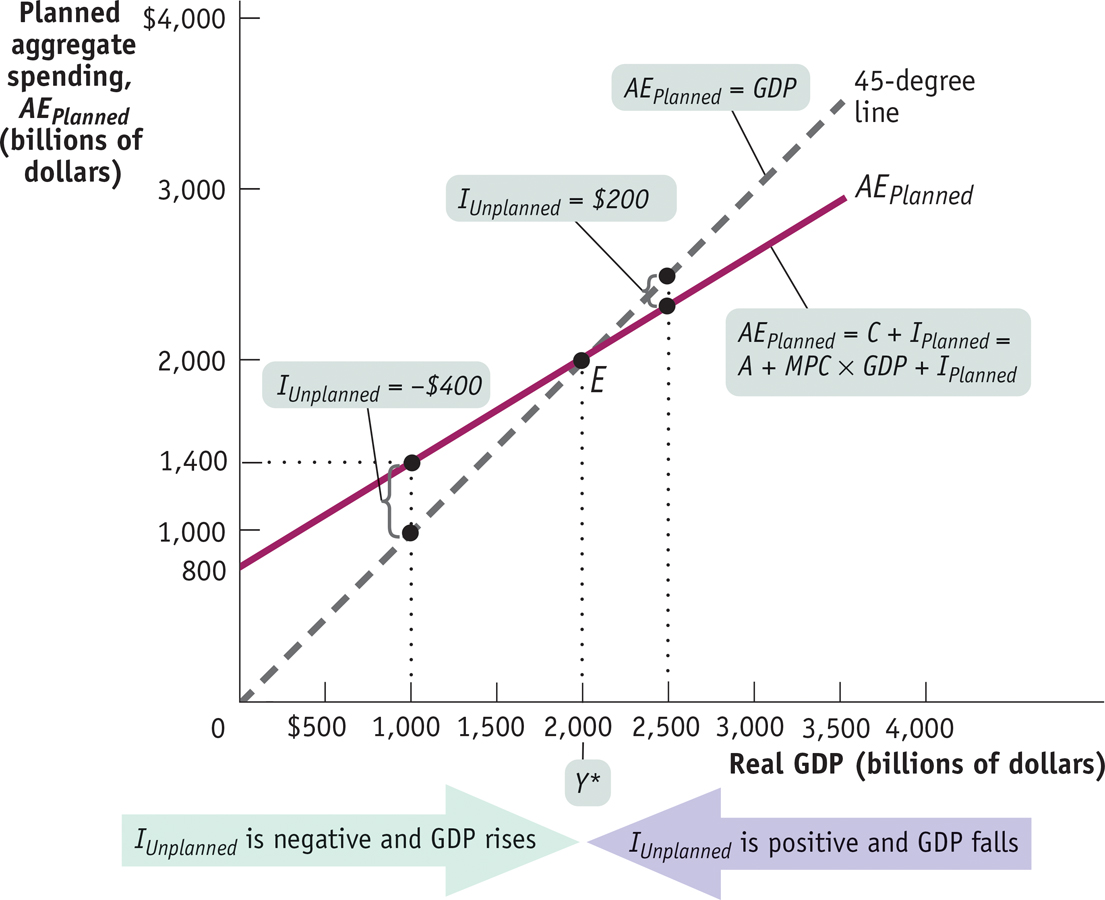
Income–Expenditure Equilibrium Income–expenditure equilibrium occurs at E, the point where the planned aggregate spending line, AEPlanned, crosses the 45-degree line. At E, the economy produces real GDP of $2,000 billion per year, the only point at which real GDP equals planned aggregate spending, AEPlanned, and unplanned inventory investment, IUnplanned, is zero. This is the level of income–expenditure equilibrium GDP, Y*. At any level of real GDP less than Y*, AEPlanned exceeds real GDP. As a result, unplanned inventory investment, IUnplanned, is negative and firms respond by increasing production. At any level of real GDP greater than Y*, real GDP exceeds AEPlanned. Unplanned inventory investment, IUnplanned, is positive and firms respond by reducing production.
This line allows us to easily spot the point of income–expenditure equilibrium, which must lie on both the 45-degree line and the planned aggregate spending line. So the point of income–expenditure equilibrium is at E, where the two lines cross. And the income–expenditure equilibrium GDP, Y*, is 2,000—the same outcome we derived in Table 11-3.
Now consider what happens if the economy isn’t in income–expenditure equilibrium. We can see from Figure 11-10 that whenever real GDP is less than Y*, the planned aggregate spending line lies above the 45-degree line and AEPlanned exceeds real GDP. In this situation, IUnplanned is negative: as shown in the figure, at a real GDP of 1,000, IUnplanned is −400. As a consequence, real GDP will rise. In contrast, whenever real GDP is greater than Y*, the planned aggregate expenditure line lies below the 45-degree line. Here, IUnplanned is positive: as shown, at a real GDP of 2,500, IUnplanned is 200. The unanticipated accumulation of inventory leads to a fall in real GDP.
The Keynesian cross diagram identifies income–expenditure equilibrium as the point where the planned aggregate spending line crosses the 45-degree line.
The type of diagram shown in Figure 11-10, which identifies income–expenditure equilibrium as the point at which the planned aggregate spending line crosses the 45-degree line, has a special place in the history of economic thought. Known as the Keynesian cross, it was developed by Paul Samuelson, one of the greatest economists of the twentieth century (as well as a Nobel Prize winner), to explain the ideas of John Maynard Keynes, the founder of macroeconomics as we know it.