1. Question 11.14

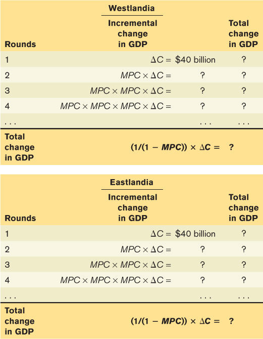
   Due to an increase in consumer wealth, there is a $40 billion autonomous increase in consumer spending in the economies of Westlandia and Eastlandia. Assuming that the aggregate price level is constant, the interest rate is fixed in both countries, and there are no taxes and no foreign trade, complete the accompanying tables to show the various rounds of increased spending that will occur in both economies if the marginal propensity to consume is 0.5 in Westlandia and 0.75 in Eastlandia. What do your results indicate about the relationship between the size of the marginal propensity to consume and the multiplier?

   

2. Question 11.15

   Assuming that the aggregate price level is constant, the interest rate is fixed, and there are no taxes and no foreign trade, what will be the change in GDP if the following events occur?

   1. There is an autonomous increase in consumer spending of $25 billion; the marginal propensity to consume is 2/3.

   2. Firms reduce investment spending by $40 billion; the marginal propensity to consume is 0.8.

   3. The government increases its purchases of military equipment by $60 billion; the marginal propensity to consume is 0.6.

3. Question 11.16

   Economists observed the only five residents of a very small economy and estimated each one’s consumer spending at various levels of current disposable income. The accompanying table shows each resident’s consumer spending at three income levels.

   Individual consumer spending by	Individual current disposable income
   	$0	$20,000	$40,000
   Andre	1,000	$15,000	29,000
   Barbara	2,500	12,500	22,500
   Casey	2,000	20,000	38,000
   Declan	5,000	17,000	29,000
   Elena	4,000	19,000	34,000

   1. What is each resident’s consumption function? What is the marginal propensity to consume for each resident?

   2. What is the economy’s aggregate consumption function? What is the marginal propensity to consume for the economy?

4. Question 11.17

   From 2009 to 2014, Eastlandia experienced large fluctuations in both aggregate consumer spending and disposable income, but wealth, the interest rate, and expected future disposable income did not change. The accompanying table shows the level of aggregate consumer spending and disposable income in millions of dollars for each of these years. Use this information to answer the following questions.

   Year	Disposable income (millions of dollars)	Consumer spending (millions of dollars)
   2009	$100	$180
   2010	350	380
   2011	300	340
   2012	400	420
   2013	375	400
   2014	500	500

   1. Plot the aggregate consumption function for Eastlandia.

   2. What is the marginal propensity to consume? What is the marginal propensity to save?

   3. What is the aggregate consumption function?

5. Question 11.18

   The Bureau of Economic Analysis reported that, in real terms, overall consumer spending increased by $66.2 billion during the second quarter of 2014.

   1. If the marginal propensity to consume is 0.52, by how much will real GDP change in response?

   2. If there are no other changes to autonomous spending other than the increase in consumer spending in part a, and unplanned inventory investment, I_Unplanned, decreased by $50 billion, what is the change in real GDP?

   3. GDP at the end of the first quarter in 2014 was $16,014.1 billion. If GDP were to increase by the amount calculated in part b, what would be the percent increase in GDP?

6. Question 11.19

   During the early 2000s, the Case–Shiller U.S. Home Price Index, a measure of average home prices, rose continuously until it peaked in March 2006. From March 2006 to May 2009, the index lost 32% of its value. Meanwhile, the stock market experienced similar ups and downs. From March 2003 to October 2007, the Standard and Poor’s 500 (S&P 500) stock index, a broad measure of stock market prices, almost doubled, from 800.73 to a high of 1,565.15. From that time until March 2009, the index fell by almost 60%, to a low of 676.53. How do you think the movements in home prices both influenced the growth in real GDP during the first half of the decade and added to the concern about maintaining consumer spending after the collapse in the housing market that began in 2006? To what extent did the movements in the stock market hurt or help consumer spending?

7. Question 11.20

   How will planned investment spending change as the following events occur?

   1. The interest rate falls as a result of Federal Reserve policy.

   2. The U.S. Environmental Protection Agency decrees that corporations must upgrade or replace their machinery in order to reduce their emissions of sulfur dioxide.

   3. Baby boomers begin to retire in large numbers and reduce their savings, resulting in higher interest rates.

8. Question 11.21

   Explain how each of the following actions will affect the level of planned investment spending and unplanned inventory investment. Assume the economy is initially in income–expenditure equilibrium.

   1. The Federal Reserve raises the interest rate.

   2. There is a rise in the expected growth rate of real GDP.

   3. A sizable inflow of foreign funds into the country lowers the interest rate.

9. Question 11.22

   In an economy with no government and no foreign sectors, autonomous consumer spending is $250 billion, planned investment spending is $350 billion, and the marginal propensity to consume is 2/3.

   1. Plot the aggregate consumption function and planned aggregate spending.

   2. What is unplanned inventory investment when real GDP equals $600 billion?

   3. What is Y*, income–expenditure equilibrium GDP?

   4. What is the value of the multiplier?

   5. If planned investment spending rises to $450 billion, what will be the new Y*?

10. Question 11.23

    An economy has a marginal propensity to consume of 0.5, and Y*, income–expenditure equilibrium GDP, equals $500 billion. Given an autonomous increase in planned investment of $10 billion, show the rounds of increased spending that take place by completing the accompanying table. The first and second rows are filled in for you. In the first row, the increase of planned investment spending of $10 billion raises real GDP and YD by $10 billion, leading to an increase in consumer spending of $5 billion (MPC × change in disposable income) in row 2, raising real GDP and YD by a further $5 billion.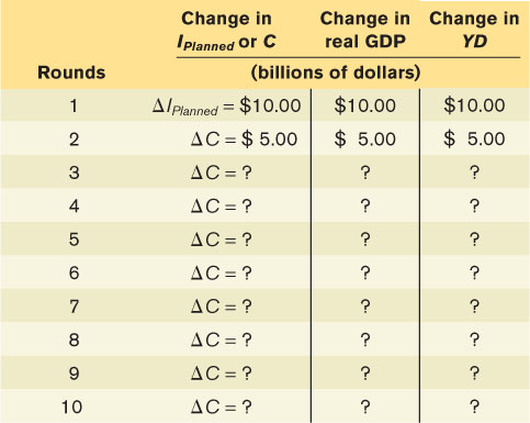

    

    1. What is the total change in real GDP after the 10 rounds? What is the value of the multiplier? What would you expect the total change in Y* to be based on the multiplier formula? How do your answers to the first and third questions compare?

    2. Redo the table starting from round 2, assuming the marginal propensity to consume is 0.75. What is the total change in real GDP after 10 rounds? What is the value of the multiplier? As the marginal propensity to consume increases, what happens to the value of the multiplier?

11. Question 11.24

    Although the United States is one of the richest nations in the world, it is also the world’s largest debtor nation. We often hear that the problem is the nation’s low savings rate. Suppose policy makers attempt to rectify this by encouraging greater savings in the economy. What effect will their successful attempts have on real GDP?

12. Question 11.25

    The U.S. economy slowed significantly in early 2008, and policy makers were extremely concerned about growth. To boost the economy, Congress passed several relief packages (the Economic Stimulus Act of 2008 and the American Recovery and Reinvestment Act of 2009) that combined would deliver about $700 billion in government spending. Assume, for the sake of argument, that this spending was in the form of payments made directly to consumers. The objective was to boost the economy by increasing the disposable income of American consumers.

    1. Calculate the initial change in aggregate consumer spending as a consequence of this policy measure if the marginal propensity to consume (MPC) in the United States is 0.5. Then calculate the resulting change in real GDP arising from the $700 billion in payments.

    2. Illustrate the effect on real GDP with the use of a graph depicting the income–expenditure equilibrium. Label the vertical axis “Planned aggregate spending, AE_Planned” and the horizontal axis “Real GDP.” Draw two planned aggregate expenditure curves (AE_Planned1 and AE_Planned2) and a 45-degree line to show the effect of the autonomous policy change on the equilibrium.

WORK IT OUT