Shifts of the SRAS Curve
An event that shifts the short-run aggregate supply curve is a supply shock.
An event that shifts the short-run aggregate supply curve, such as a change in commodity prices, nominal wages, or productivity, is known as a supply shock. A negative supply shock raises production costs and reduces the quantity producers are willing to supply at any given aggregate price level, leading to a leftward shift of the short-run aggregate supply curve. The U.S. economy experienced severe negative supply shocks following disruptions to world oil supplies in 1973 and 1979. In contrast, a positive supply shock reduces production costs and increases the quantity supplied at any given aggregate price level, leading to a rightward shift of the short-run aggregate supply curve. The United States experienced a positive supply shock between 1995 and 2000, when the increasing use of the internet and other information technologies caused productivity growth to surge.
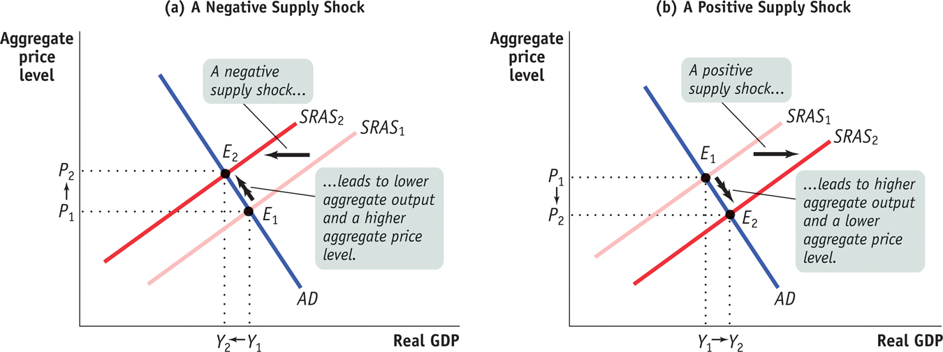
The effects of a negative supply shock are shown in panel (a) of Figure 12-13. The initial equilibrium is at E1, with aggregate price level P1 and aggregate output Y1. The disruption in the oil supply causes the short-run aggregate supply curve to shift to the left, from SRAS1 to SRAS2. As a consequence, aggregate output falls and the aggregate price level rises, an upward movement along the AD curve. At the new equilibrium, E2, the short-run equilibrium aggregate price level, P2, is higher, and the short-run equilibrium aggregate output level, Y2, is lower than before.

Supply Shocks A supply shock shifts the short-run aggregate supply curve, moving the aggregate price level and aggregate output in opposite directions. Panel (a) shows a negative supply shock, which shifts the short-run aggregate supply curve leftward and causes stagflation—lower aggregate output and a higher aggregate price level. Here the short-run aggregate supply curve shifts from SRAS1 to SRAS2, and the economy moves from E1 to E2. The aggregate price level rises from P1 to P2, and aggregate output falls from Y1 to Y2. Panel (b) shows a positive supply shock, which shifts the short-run aggregate supply curve rightward, generating higher aggregate output and a lower aggregate price level. The short-run aggregate supply curve shifts from SRAS1 to SRAS2, and the economy moves from E1 to E2. The aggregate price level falls from P1 to P2, and aggregate output rises from Y1 to Y2.
Stagflation is the combination of inflation and falling aggregate output.
The combination of inflation and falling aggregate output shown in panel (a) has a special name: stagflation, for “stagnation plus inflation.” When an economy experiences stagflation, it’s very unpleasant: falling aggregate output leads to rising unemployment, and people feel that their purchasing power is squeezed by rising prices. Stagflation in the 1970s led to a mood of national pessimism. It also, as we’ll see shortly, poses a dilemma for policy makers.
A positive supply shock, shown in panel (b), has exactly the opposite effects. A rightward shift of the SRAS curve from SRAS1 to SRAS2 results in a rise in aggregate output and a fall in the aggregate price level, a downward movement along the AD curve. The favorable supply shocks of the late 1990s led to a combination of full employment and declining inflation. That is, the aggregate price level fell compared with the long-run trend. This combination produced, for a time, a great wave of national optimism.
The distinctive feature of supply shocks, both negative and positive, is that, unlike demand shocks, they cause the aggregate price level and aggregate output to move in opposite directions.
There’s another important contrast between supply shocks and demand shocks. As we’ve seen, monetary policy and fiscal policy enable the government to shift the AD curve, meaning that governments are in a position to create the kinds of shocks shown in Figure 12-12. It’s much harder for governments to shift the AS curve. Are there good policy reasons to shift the AD curve? We’ll turn to that question soon. First, however, let’s look at the difference between short-run macroeconomic equilibrium and long-run macroeconomic equilibrium.
Supply Shocks of the Twenty-first Century
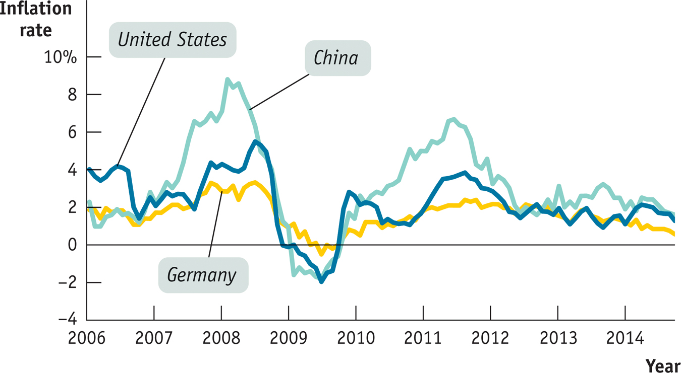
The price of oil and other raw materials has been highly unstable in recent years, with surging prices in 2007–2008, plunging prices in 2008–2009, and another surge starting in the second half of 2010. The reasons for these wild swings are somewhat controversial, but their macroeconomic implications are clear: much of the world has been subjected to a series of supply shocks. There was a negative shock in 2007–2008, a positive shock in 2008–2009, and another negative shock in 2010–2011.
You can see the effect of these shocks in the accompanying figure, which shows the rate of inflation, as measured by the percentage change in consumer prices over the previous year, in three large economies. Economic policies have been quite different in the United States, Germany (which shares a currency with many other European countries), and China. Yet in all three inflation rose sharply in 2007–2008, fell dramatically thereafter, and rose sharply again in 2011.
Source: Federal Reserve Bank of St. Louis.

