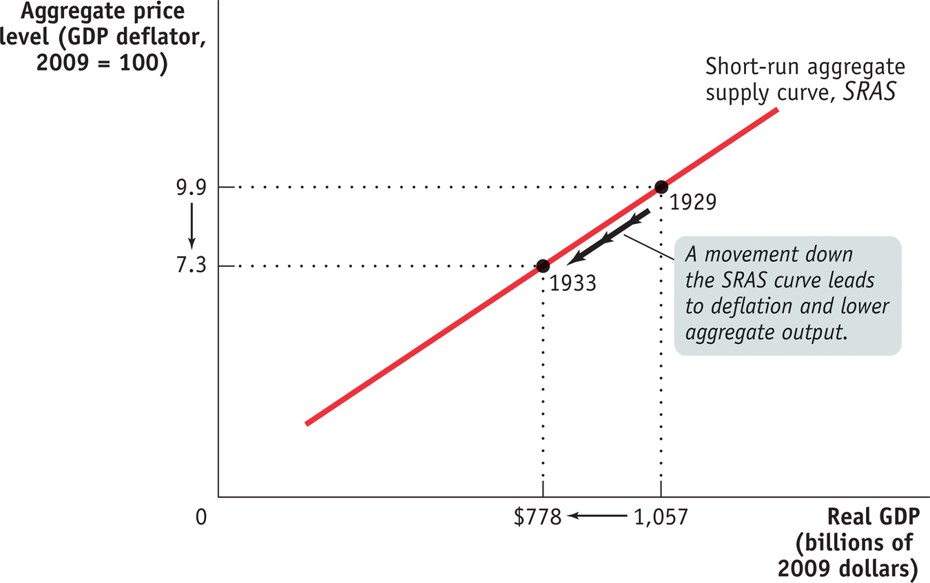
The period from 1929 to 1933 demonstrated that there is a positive relationship in the short run between the aggregate price level and the quantity of aggregate output supplied. That is, a rise in the aggregate price level is associated with a rise in the quantity of aggregate output supplied, other things equal; a fall in the aggregate price level is associated with a fall in the quantity of aggregate output supplied, other things equal. To understand why this positive relationship exists, consider the most basic question facing a producer: is producing a unit of output profitable or not? Let’s define profit per unit:

Thus, the answer to the question depends on whether the price the producer receives for a unit of output is greater or less than the cost of producing that unit of output. At any given point in time, many of the costs producers face are fixed per unit of output and can’t be changed for an extended period of time. Typically, the largest source of inflexible production cost is the wages paid to workers. Wages here refers to all forms of worker compensation, such as employer-paid health care and retirement benefits in addition to earnings.

Wages are typically an inflexible production cost because the dollar amount of any given wage paid, called the nominal wage, is often determined by contracts that were signed some time ago. And even when there are no formal contracts, there are often informal agreements between management and workers, making companies reluctant to change wages in response to economic conditions. For example, companies usually will not reduce wages during poor economic times—unless the downturn has been particularly long and severe—for fear of generating worker resentment. Correspondingly, they typically won’t raise wages during better economic times—until they are at risk of losing workers to competitors—because they don’t want to encourage workers to routinely demand higher wages.

As a result of both formal and informal agreements, then, the economy is characterized by sticky wages: nominal wages that are slow to fall even in the face of high unemployment and slow to rise even in the face of labor shortages. It’s important to note, however, that nominal wages cannot be sticky forever: ultimately, formal contracts and informal agreements will be renegotiated to take into account changed economic circumstances. As the Pitfalls at the end of this section explains, how long it takes for nominal wages to become flexible is an integral component of what distinguishes the short run from the long run.

To understand how the fact that many costs are fixed in nominal terms gives rise to an upward-sloping short-run aggregate supply curve, it’s helpful to know that prices are set somewhat differently in different kinds of markets. In perfectly competitive markets, producers take prices as given; in imperfectly competitive markets, producers have some ability to choose the prices they charge. In both kinds of markets, there is a short-run positive relationship between prices and output, but for slightly different reasons.

Let’s start with the behavior of producers in perfectly competitive markets; remember, they take the price as given. Imagine that, for some reason, the aggregate price level falls, which means that the price received by the typical producer of a final good or service falls. Because many production costs are fixed in the short run, production cost per unit of output doesn’t fall by the same proportion as the fall in the price of output. So the profit per unit of output declines, leading perfectly competitive producers to reduce the quantity supplied in the short run.

On the other hand, suppose that for some reason the aggregate price level rises. As a result, the typical producer receives a higher price for its final good or service. Again, many production costs are fixed in the short run, so production cost per unit of output doesn’t rise by the same proportion as the rise in the price of a unit. And since the typical perfectly competitive producer takes the price as given, profit per unit of output rises and output increases.

Now consider an imperfectly competitive producer that is able to set its own price. If there is a rise in the demand for this producer’s product, it will be able to sell more at any given price. Given stronger demand for its products, it will probably choose to increase its prices as well as its output, as a way of increasing profit per unit of output. In fact, industry analysts often talk about variations in an industry’s “pricing power”: when demand is strong, firms with pricing power are able to raise prices—and they do.

Conversely, if there is a fall in demand, firms will normally try to limit the fall in their sales by cutting prices.

Both the responses of firms in perfectly competitive industries and those of firms in imperfectly competitive industries lead to an upward-sloping relationship between aggregate output and the aggregate price level. The positive relationship between the aggregate price level and the quantity of aggregate output producers are willing to supply during the time period when many production costs, particularly nominal wages, can be taken as fixed is illustrated by the short-run aggregate supply curve. The positive relationship between the aggregate price level and aggregate output in the short run gives the short-run aggregate supply curve its upward slope.

Figure 12-5 shows a hypothetical short-run aggregate supply curve, SRAS, which matches actual U.S. data for 1929 and 1933. On the horizontal axis is aggregate output (or, equivalently, real GDP)—the total quantity of final goods and services supplied in the economy—measured in 2009 dollars. On the vertical axis is the aggregate price level as measured by the GDP deflator, with the value for the year 2009 equal to 100. In 1929, the aggregate price level was 9.9 and real GDP was $1,057 billion. In 1933, the aggregate price level was 7.3 and real GDP was only $778 billion. The movement down the SRAS curve corresponds to the deflation and fall in aggregate output experienced over those years.