The key statistic used to track economic growth is real GDP per capita—real GDP divided by the population size. We focus on GDP because, as we learned in Chapter 7, GDP measures the total value of an economy’s production of final goods and services as well as the income earned in that economy in a given year. We use real GDP because we want to separate changes in the quantity of goods and services from the effects of a rising price level. We focus on real GDP per capita because we want to isolate the effect of changes in the population. For example, other things equal, an increase in the population lowers the standard of living for the average person—there are now more people to share a given amount of real GDP. An increase in real GDP that only matches an increase in population leaves the average standard of living unchanged.

Although we also learned in Chapter 7 that growth in real GDP per capita should not be a policy goal in and of itself, it does serve as a very useful summary measure of a country’s economic progress over time. Figure 9-1 shows real GDP per capita for the United States, India, and China, measured in 1990 dollars, from 1900 to 2010. (We’ll talk about India and China in a moment.) The vertical axis is drawn on a logarithmic scale so that equal percent changes in real GDP per capita across countries are the same size in the graph.

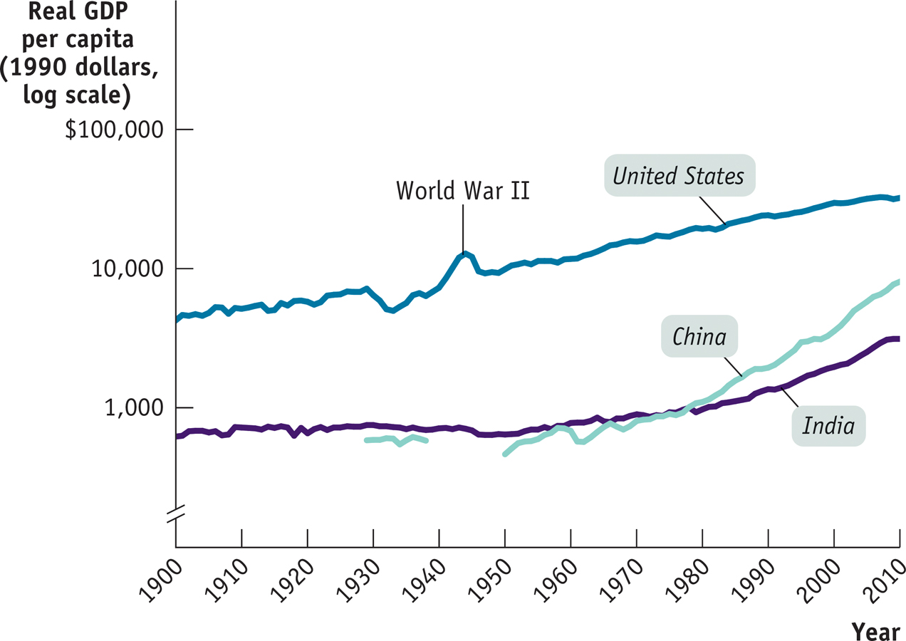
To give a sense of how much the U.S. economy grew during the last century, Table 9-1 shows real GDP per capita at selected years, expressed two ways: as a percentage of the 1900 level and as a percentage of the 2010 level. In 1920, the U.S. economy already produced 136% as much per person as it did in 1900. In 2010, it produced 758% as much per person as it did in 1900, an almost eightfold increase. Alternatively, in 1900 the U.S. economy produced only 13% as much per person as it did in 2010.

The income of the typical family normally grows more or less in proportion to per capita income. For example, a 1% increase in real GDP per capita corresponds, roughly, to a 1% increase in the income of the median or typical family—a family at the center of the income distribution. In 2010, the median American household had an income of about $50,000. Since Table 9-1 tells us that real GDP per capita in 1900 was only 13% of its 2010 level, a typical family in 1900 probably had a purchasing power only 13% as large as the purchasing power of a typical family in 2010. That’s around $6,850 in today’s dollars, representing a standard of living that we would now consider severe poverty. Today’s typical American family, if transported back to the United States of 1900, would feel quite a lot of deprivation.

Yet many people in the world have a standard of living equal to or lower than that of the United States at the beginning of the last century. That’s the message about China and India in Figure 9-1: despite dramatic economic growth in China over the last three decades and the less dramatic acceleration of economic growth in India, China has only recently exceeded the standard of living that the United States enjoyed in the early twentieth century, while India is still poorer than the United States was at that time. And much of the world today is poorer than China or India.

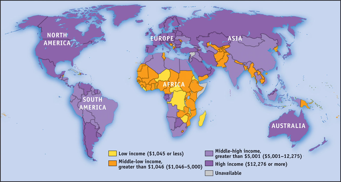
You can get a sense of how poor much of the world remains by looking at Figure 9-2, a map of the world in which countries are classified according to their 2013 levels of GDP per capita, in U.S. dollars. As you can see, large parts of the world have very low incomes. Generally speaking, the countries of Europe and North America, as well as a few in the Pacific, have high incomes. The rest of the world, containing most of its population, is dominated by countries with GDP less than $5,000 per capita—and often much less. In fact, today about 50% of the world’s people live in countries with a lower standard of living than the United States had a century ago.