1.2 Module 37: Externalities and Public Policy

© Accent Alaska.com/Alamy

Policies Toward Pollution

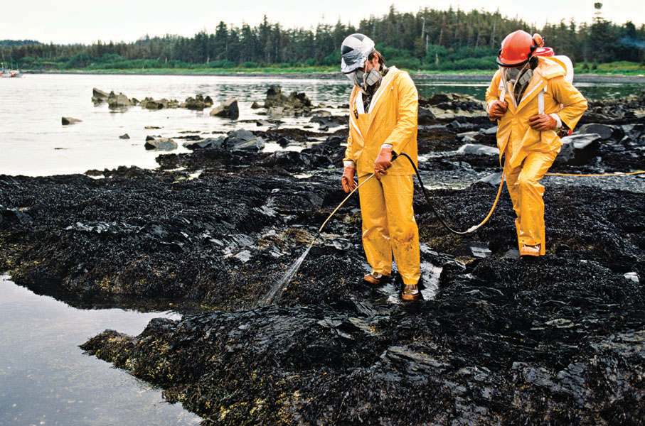
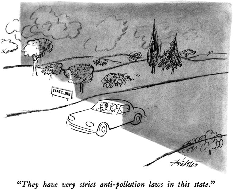
Before 1970 there were no rules governing the amount of sulfur dioxide that power plants in the United States could emit—which is why acid rain got to be such a problem. In 1970, the Clean Air Act set rules about sulfur dioxide emissions; thereafter, the acidity of rainfall declined significantly. Economists argued, however, that a more flexible system of rules that exploited the effectiveness of markets could achieve lower pollution levels at a lower cost. In 1990 this theory was put into effect with a modified version of the Clean Air Act. And guess what? The economists were right!

In this module we’ll look at the three types of policies governments typically use to deal with pollution:

1. Environmental standards
2. Emissions taxes
3. Tradable emissions permits

We’ll also see how economic analysis has been used to improve those policies.

Environmental Standards

Because the economy, and life itself, depends on a viable environment, external costs that threaten the environment—air pollution, water pollution, habitat destruction, and so on, are worthy of attention. Protection of the environment has become a major focus of government in every advanced nation. In the United States, the Environmental Protection Agency is the principal enforcer of environmental policies at the national level and is supported by the actions of state and local governments.

How does a country protect its environment? At present the main policy tools are environmental standards, rules that protect the environment by specifying actions by producers and consumers. A familiar example is the law that requires almost all vehicles to have catalytic converters, which reduce the emission of chemicals that can cause smog and lead to health problems. Other rules require communities to treat their sewage, factories to limit their pollution emissions, and homes to be painted with lead-free paint, among many other examples.

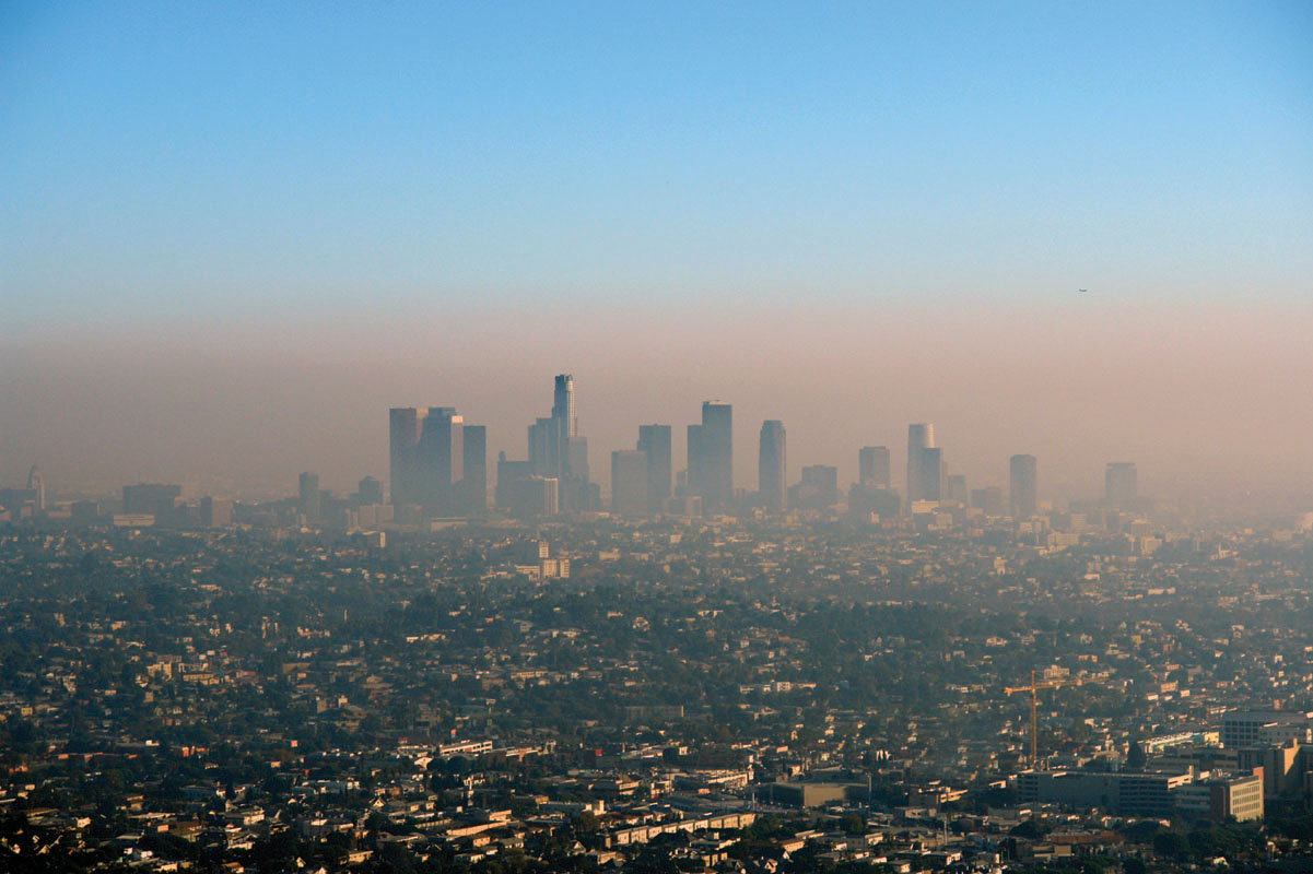
Environmental standards came into widespread use in the 1960s and 1970s with considerable success. Since the United States passed the Clean Air Act in 1970, for example, the emission of air pollutants has fallen by more than a third, even though the population has grown by a third and the size of the economy has more than doubled. Even in Los Angeles, still famous for its smog, the air has improved dramatically: in 1976 ozone levels in the South Coast Air Basin exceeded federal standards on 194 days; in 2010, on only 7 days. Improvements have continued in 2013.

Despite these successes, economists believe that when regulators can control a polluter’s emissions directly, there are more efficient ways than environmental standards to deal with pollution. By using methods grounded in economic analysis, society can achieve a cleaner environment at lower cost.

Environmental standards have helped reduce the Los Angeles smog and improve air quality.

iStockphoto

Most current environmental standards are inflexible and don’t allow reductions in pollution to be achieved at the lowest possible cost. For example, two power plants—plant A and plant B—might be ordered to reduce pollution by the same percentage, even if their costs of achieving that objective are very different.

How does economic theory suggest that pollution should be controlled? We’ll examine two approaches: taxes and tradable permits. As we’ll see, either approach can achieve the efficient outcome at the minimum feasible cost.

Emissions Taxes

One way to deal with pollution directly is to charge polluters an emissions tax. Emissions taxes depend on the amount of pollution a firm produces. For example, power plants might be charged $200 for every ton of sulfur dioxide they emit.

Consider the socially optimal quantity of pollution, Q_OPT, shown in Figure 37-1. At that quantity of pollution, the marginal social benefit and the marginal social cost of an additional ton of emissions are equal at $200. But in the absence of government intervention, power companies have no incentive to limit pollution to the socially optimal quantity Q_OPT; instead, they will push pollution up to the quantity Q_MKT, at which the marginal social benefit is zero.

The market determined quantity of pollution, Q_MKT, is too high because polluters don’t pay the marginal social cost, and thus pollute beyond the socially optimal quantity, Q_OPT, at which marginal social cost equals marginal social benefit. A Pigouvian tax of $200—the value of the marginal social cost of pollution when it equals the marginal social benefit of pollution—gives polluters the incentive to emit only the socially optimal quantity of pollution. Another solution is to provide permits for only the socially optimal quantity of pollution.

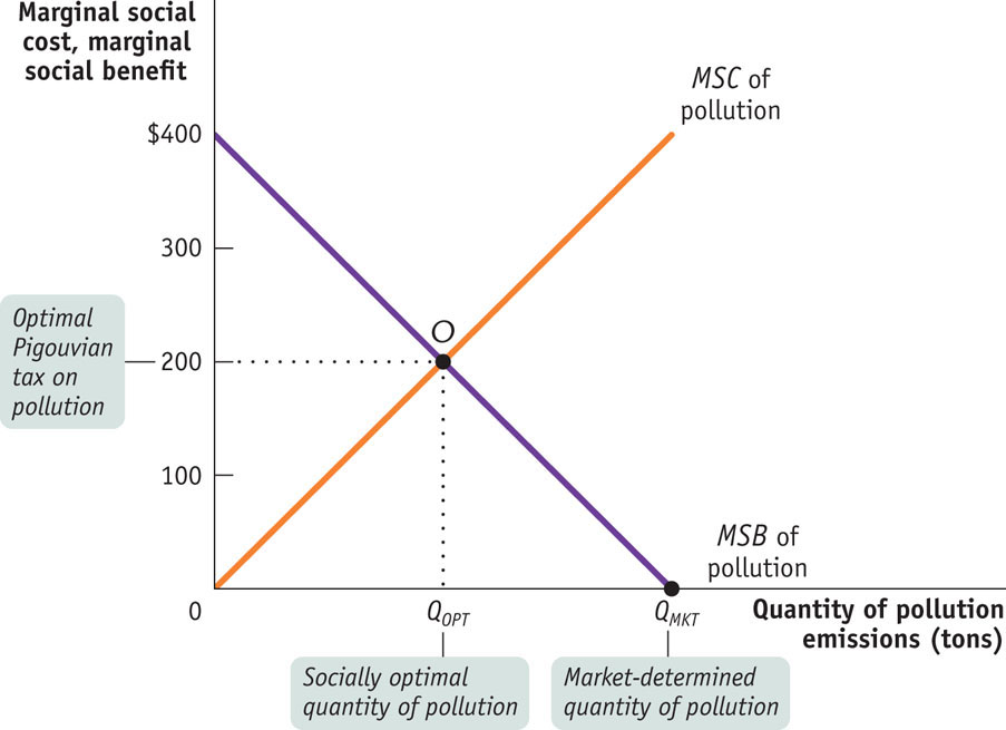
It’s now easy to see how an emissions tax can solve the problem. If power companies are required to pay a tax of $200 per ton of emissions, they face a marginal cost of $200 per ton and have an incentive to reduce emissions to Q_OPT, the socially optimal quantity. This illustrates a general result: an emissions tax equal to the marginal social cost at the socially optimal quantity of pollution induces polluters to internalize the externality—to take into account the true cost to society of their actions. (The Pigouvian tax noted in Figure 37-1 will be explained shortly.)

Why is an emissions tax an efficient way (that is, a cost-minimizing way) to reduce pollution but environmental standards generally are not? Because an emissions tax ensures that the marginal benefit of pollution is equal for all sources of pollution, but an environmental standard does not.

Figure 37-2 shows a hypothetical industry consisting of only two plants, plant A and plant B. We’ll assume that plant A uses newer technology than plant B and so has a lower cost of reducing pollution. Reflecting this difference in costs, plant A’s marginal benefit of pollution curve, MB_A, lies below plant B’s marginal benefit of pollution curve, MB_B. Because it is more costly for plant B to reduce its pollution at any output quantity, an additional ton of pollution is worth more to plant B than to plant A.

In both panels, MB_A shows the marginal benefit of pollution to plant A and MB_B shows the marginal benefit of pollution to plant B. In the absence of government intervention, each plant would emit 600 tons. However, the cost of reducing emissions is lower for plant A, as shown by the fact that MB_A lies below MB_B. Panel (a) shows the result of an environmental standard that requires both plants to cut emissions in half; this is inefficient, because it leaves the marginal benefit of pollution higher for plant B than for plant A. Panel (b) shows that an emissions tax achieves the same quantity of overall pollution efficiently: faced with an emissions tax of $200 per ton, both plants reduce pollution to the point where its marginal benefit is $200.

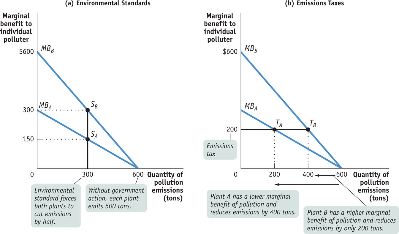
In the absence of government action, polluters will pollute until the marginal social benefit of an additional unit of emissions is equal to zero. Recall that the marginal social benefit of pollution is the cost savings, at the margin, to polluters of an additional unit of pollution. As a result, without government intervention each plant will pollute until its own marginal benefit of pollution is equal to zero. This corresponds to an emissions quantity of 600 tons each for plants A and B—the quantity of pollution at which MB_A and MB_B are each equal to zero. So although plant A and plant B value a ton of emissions differently, without government action they will each choose to emit the same amount of pollution.

Now suppose that the government decides that overall pollution from this industry should be cut in half, from 1,200 tons to 600 tons. Panel (a) of Figure 37-2 shows how this might be achieved with an environmental standard that requires each plant to cut its emissions in half, from 600 to 300 tons. The standard has the desired effect of reducing overall emissions from 1,200 to 600 tons but accomplishes it in an inefficient way. As you can see from panel (a), the environmental standard leads plant A to produce at point S_A, where its marginal benefit of pollution is $150, but plant B produces at point S_B, where its marginal benefit of pollution is twice as high, $300.

This difference in marginal benefits between the two plants tells us that the same quantity of pollution can be achieved at lower total cost by allowing plant B to pollute more than 300 tons but inducing plant A to pollute less. In fact, the efficient way to reduce pollution is to ensure that at the industry-wide outcome, the marginal benefit of pollution is the same for all plants. When each plant values a unit of pollution equally, there is no way to rearrange pollution reduction among the various plants that achieves the optimal quantity of pollution at a lower total cost.

© Mischa Richter/The New Yorker Collection/www.cartoonbank.com

We can see from panel (b) how an emissions tax achieves exactly that result. Suppose both plant A and plant B pay an emissions tax of $200 per ton so that the marginal cost of an additional ton of emissions to each plant is now $200 rather than zero. As a result, plant A produces at T_A and plant B produces at T_B. So plant A reduces its pollution more than it would under an inflexible environmental standard, cutting its emissions from 600 to 200 tons; meanwhile, plant B reduces its pollution less, going from 600 to 400 tons. In the end, total pollution—600 tons—is the same as under the environmental standard, but total surplus is higher. That’s because the reduction in pollution has been achieved efficiently, allocating most of the reduction to plant A, the plant that can reduce emissions at lower cost.

The term emissions tax may convey the misleading impression that taxes are a solution to only one kind of external cost, pollution. In fact, taxes can be used to discourage any activity that generates negative externalities, such as driving during rush hour or operating a noisy bar in a residential area. In general, taxes designed to reduce external costs are known as Pigouvian taxes, after the economist A.C. Pigou, who emphasized their usefulness in a classic 1920 book, The Economics of Welfare. Look again at Figure 37-1. In our example, the optimal Pigouvian tax is $200; this corresponds to the marginal social cost of pollution at the optimal output quantity, Q_OPT.

Are there any problems with emissions taxes? The main concern is that in practice government officials usually aren’t sure at what level the tax should be set. If they set the tax too low, improvement in the environment will be inadequate; if they set it too high, emissions will be reduced by more than is efficient. This uncertainty cannot be eliminated, but the nature of the risks can be changed by using an alternative strategy, issuing tradable emissions permits.

Tradable Emissions Permits

Tradable emissions permits are licenses to emit limited quantities of pollutants that can be bought and sold by polluters. They are usually issued to polluting firms according to some formula reflecting their history. For example, each power plant might be issued permits equal to 50% of its emissions before the system went into effect. The more important point, however, is that these permits are tradable. Firms with differing costs of reducing pollution can now engage in mutually beneficial transactions: those that find it easier to reduce pollution will sell some of their permits to those that find it more difficult.

In other words, firms will use transactions in permits to reallocate pollution reduction among themselves, so that in the end those with the lowest cost will reduce their pollution the most and those with the highest cost will reduce their pollution the least. Assume that the government issues 300 permits each to plant A and plant B, where one permit allows the emission of one ton of pollution. Under a system of tradable emissions permits, commonly known as a cap and trade program, plant A will find it profitable to sell 100 of its 300 government-issued permits to plant B. The effect of a cap and trade program is to create a market in rights to pollute.

Just like emissions taxes, tradable permits provide polluters with an incentive to take the marginal social cost of pollution into account. To see why, suppose that the market price of a permit to emit one ton of sulfur dioxide is $200. Then every plant has an incentive to limit its emissions of sulfur dioxide to the point where its marginal benefit of emitting another ton of pollution is $200. This is obvious for plants that buy rights to pollute: if a plant must pay $200 for the right to emit an additional ton of sulfur dioxide, it faces the same incentives as a plant facing an emissions tax of $200 per ton.

But it’s equally true for plants that have more permits than they plan to use: by not emitting a ton of sulfur dioxide, a plant frees up a permit that it can sell for $200, so the opportunity cost of a ton of emissions to the plant’s owner is $200.

In short, tradable emissions permits have the same cost-minimizing advantage as emissions taxes over environmental standards: either system ensures that those who can reduce pollution most cheaply are the ones who do so. The socially optimal quantity of pollution shown in Figure 37-1 could be efficiently achieved either way: by imposing an emissions tax of $200 per ton of pollution or by issuing tradable permits to emit Q_OPT tons of pollution. If regulators choose to issue Q_OPT permits, where one permit allows the release of one ton of emissions, then the equilibrium market price of a permit among polluters will indeed be $200. Why? You can see from Figure 37-1 that at Q_OPT, only polluters with a marginal benefit of pollution of $200 or more will buy a permit. And the last polluter who buys—who has a marginal benefit of exactly $200—sets the market price.

It’s important to realize that emissions taxes and tradable permits do more than induce polluting industries to reduce their output. Unlike rigid environmental standards, emissions taxes and tradable permits provide incentives to create and use technology that emits less pollution—new technology that lowers the socially optimal level of pollution. The main effect of the permit system for sulfur dioxide has been to change how electricity is produced rather than to reduce the nation’s electricity output. For example, power companies have shifted to the use of alternative fuels such as low-sulfur coal and natural gas; they have also installed scrubbers that take much of the sulfur dioxide out of a power plant’s emissions.

The main problem with tradable emissions permits is the flip-side of the problem with emissions taxes: because it is difficult to determine the optimal quantity of pollution, governments can find themselves either issuing too many permits (that is, they don’t reduce pollution enough) or issuing too few (that is, they reduce pollution too much).

After first relying on environmental standards, the U.S. government has turned to a system of tradable permits to control acid rain. Current proposals would extend the system to other major sources of pollution. And in 2005 the European Union created an emissions-trading scheme with the purpose of controlling emissions of carbon dioxide, a greenhouse gas. The European Union scheme is part of a larger global market for the trading of greenhouse gas permits. The Economics in Action that follows describes these two systems in greater detail.

!world_eia!CAP AND TRADE

The tradable emissions permit systems for both acid rain in the United States and greenhouse gases in the European Union are examples of cap and trade systems: the government sets a cap (a maximum amount of pollutant that can be emitted), issues tradable emissions permits, and enforces a yearly rule that a polluter must hold a number of permits equal to the amount of pollutant emitted. The goal is to set the cap low enough to generate environmental benefits, while giving polluters flexibility in meeting environmental standards and motivating them to adopt new technologies that will lower the cost of reducing pollution.

In 1994 the United States began a cap and trade system for the sulfur dioxide emissions that cause acid rain by issuing permits to power plants based on their historical consumption of coal. Thanks to the system, air pollutants in the United States decreased by more than 40% from 1990 to 2008, and 2010 acid rain levels dropped to approximately 50% of their 1980 levels and they continue to drop.

Economists who have analyzed the sulfur dioxide cap and trade system point to another reason for its success: it would have been a lot more expensive—80% more to be exact—to reduce emissions by this much using a non-market-based regulatory policy.

Cap and trade systems can benefit the environment, but they are not a silver bullet against pollution.

AP Photo/Kin Cheung

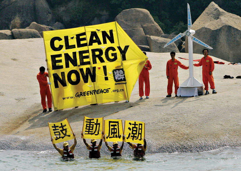
The EU cap and trade scheme, covering all 28 member nations of the European Union (plus Iceland, Liechtenstein, and Norway), is the world’s only mandatory trading scheme for greenhouse gases. It is scheduled to achieve a 21% reduction in greenhouse gases by 2020 compared to 2005 levels.

Despite all this good news, however, cap and trade systems are not silver bullets for the world’s pollution problems for these reasons:

• Although they are appropriate for pollution that’s geographically dispersed, like sulfur dioxide and greenhouse gases, they don’t work for pollution that’s localized, like mercury or lead contamination.
• The amount of overall reduction in pollution depends on the level of the cap. Under industry pressure, regulators run the risk of issuing too many permits, effectively eliminating the cap.
• There must be vigilant monitoring of compliance if the system is to work. Without oversight of a polluter’s emissions, there is no way to know for sure that the rules are being followed.

Positive Externalities

New Jersey is the most densely populated state in the country, lying along the northeastern corridor, an area of almost continuous development stretching from Washington, D.C., to Boston. Yet a drive through New Jersey reveals a surprising feature: acre upon acre of farmland, growing everything from corn to pumpkins to the famous Jersey tomatoes. This situation is no accident: starting in 1961, New Jerseyans have voted in a series of measures that subsidize farmers to permanently preserve their farmland rather than sell it to developers.

Why have New Jersey citizens voted to raise their own taxes to subsidize the preservation of farmland? Because they believe that preserved farmland in an already heavily developed state provides external benefits, such as natural beauty, access to fresh food, and the conservation of wild bird populations. In addition, preservation alleviates the external costs that come with more development, such as pressure on roads, water supplies, and municipal services—and, inevitably, more pollution.

In this section we’ll explore the topics of external benefits and positive externalities. They are, in many ways, the mirror images of external costs and negative externalities. Left on its own, the market will produce too little of a good (in this case, preserved New Jersey farmland) that confers external benefits on others. But society as a whole is better off when policies are adopted that increase the supply of such a good.

Preserved Farmland: An External Benefit

Preserved farmland yields both benefits and costs to society. In the absence of government intervention, the farmer who wants to sell his land incurs all the costs of preservation—namely, the forgone profit to be made from selling the farmland to a developer. But the benefits of preserved farmland accrue not to the farmer but to neighboring residents, who have no right to influence how the farmland is disposed of.

Preserved farmland provides external benefits to an entire community.

© Gene Ahrens/Alamy

Figure 37-3 illustrates society’s problem. The marginal social cost of preserved farmland, shown by the MSC curve, is the additional cost imposed on society by an additional acre of such farmland. This represents the forgone profits that would have accrued to farmers if they had sold their land. The line is upward-sloping because when very few acres are preserved and there is plenty of land available for development, the profit that could be made from selling an acre to a developer is small. But as the number of preserved acres increases and few are left for development, the amount a developer is willing to pay for them, and therefore the forgone profit, increases as well.

The MSB curve represents the marginal social benefit of preserved farmland. It is the additional benefit that accrues to society—in this case, the farmer’s neighbors—when an additional acre of farmland is preserved. The curve is downward sloping because as more farmland is preserved, the benefit to society of preserving another acre falls. As Figure 37-3 shows, the socially optimal point, O, occurs when the marginal social cost and the marginal social benefit are equalized—here, at a price of $10,000 per acre. At the socially optimum point, Q_OPT acres of farmland are preserved.

Without government intervention, the quantity of preserved farmland will be zero, the level at which the marginal social cost of preservation is zero. This is an inefficiently low quantity of preserved farmland: the marginal social benefit is $20,000, but the marginal social cost is zero. An optimal Pigouvian subsidy of $10,000, the value of the marginal social benefit of preservation when it equals the marginal social cost, can move the market to the socially optimal level of preservation, Q_OPT.

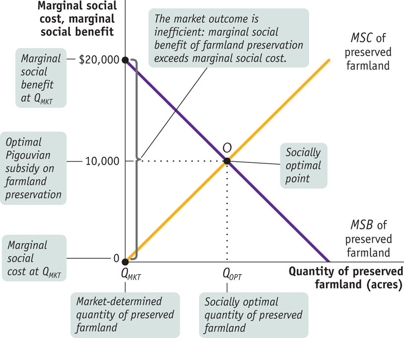
The market alone will not provide Q_OPT acres of preserved farmland. Instead, in the market outcome no acres will be preserved; the level of preserved farmland, Q_MKT, is equal to zero. That’s because farmers will set the marginal social cost of preservation—their forgone profits—at zero and sell all their acres to developers. Because farmers bear the entire cost of preservation but gain none of the benefits, an inefficiently low quantity of acres will be preserved in the market outcome.

This is clearly inefficient because at zero acres preserved, the marginal social benefit of preserving an acre of farmland is $20,000. So how can the economy be induced to produce Q_OPT acres of preserved farmland, the socially optimal level? The answer is a Pigouvian subsidy: a payment designed to encourage activities that yield external benefits. The optimal Pigouvian subsidy, as shown in Figure 37-3, is equal to the marginal social benefit of preserved farmland at the socially optimal level, Q_OPT—that is, $10,000 per acre.

So New Jersey voters are indeed implementing the right policy to raise their social welfare—taxing themselves in order to provide subsidies for farmland preservation.

Positive Externalities in the Modern Economy

In the overall U.S. economy, the most important single source of external benefits is the creation of knowledge. In high-tech industries such as semiconductors, software design, green technology, and bioengineering, innovations by one firm are quickly emulated and improved upon by rival firms. Such spreading of knowledge across individuals and firms is known as a technology spillover. In the modern economy, the greatest sources of technology spillovers are major universities and research institutes.

Informal interactions can lead to technological innovation.

Creatista/Shutterstock

In technologically advanced countries such as the United States, Japan, the United Kingdom, Germany, France, and Israel, there is an ongoing exchange of people and ideas among private industries, major universities, and research institutes located in close proximity. The dynamic interplay that occurs in these research clusters spurs innovation and competition, theoretical advances, and practical applications. (See the Business Case at the end of the section for more on research clusters.) Ultimately, these areas of technology spillover increase the economy’s productivity and raise living standards.

But research clusters don’t appear out of thin air. Except in a few instances in which firms have funded basic research on a long-term basis, research clusters have grown up around major universities. And like farmland preservation in New Jersey, major universities and their research activities are subsidized by government. In fact, government policy makers in advanced countries have long understood that the external benefits generated by knowledge, stemming from basic education to high-tech research, are key to the economy’s growth over time.

Network Externalities

Unlike positive externalities, network externalities have no inherently favorable or adverse effect on society at large. They do, however, affect other users of the associated good or service. Consider Facebook again: if you were the only user of Facebook, what would it be worth to you? The answer, of course, is nothing. Facebook derives its value only from the fact that other people also use it. And the more people who use Facebook, the more valuable it is to you.

A network externality exists when the value of a good or service to an individual is greater when a large number of other people also use the good or service. Although network externalities are common in technology-driven sectors of the economy, the phenomenon is much more widespread than that.

For all network externalities, the value of the good or service is derived entirely from its ability to link many people possessing the same good or service. As a result, the marginal benefit of the good or service to any one individual depends on the number of other individuals who use it.

Although most network externalities involve methods of communication—the Internet and cell phones, for example—they can exist when other users are not strictly necessary for the use of a good, as long as they enhance its usefulness. For example, a scheduled flight between two airports becomes more valuable if one or both of those airports is a hub with connections to other places.

Even your choice of a car is influenced by a form of network externality. Most people would be reluctant to switch to a car that runs on natural gas because fueling the car would be difficult: very few gas stations offer natural gas. And the reason service stations do not offer natural gas is, of course, that few people drive anything other than gasoline-powered cars.

When a good or service is subject to a network externality, it exhibits positive feedback: if large numbers of people buy it, other people become more likely to buy it, too. If people don’t buy the good or service, others become less likely to buy it. So both success and failure tend to be self-reinforcing. Producers of products that are subject to network externalities are aware of this problem, understanding that of two competing products, it’s the one with the largest network—not necessarily the one that’s the better product—that will win in the end. That is, the product with the largest network will eventually dominate the market, and competing products will eventually disappear.

Module 37 Review

Check Your Understanding

The use of plastic water bottles creates a negative externality by increasing pollution and the amount of material sent into a landfill. Suppose we imposed a tax of $0.50 for each water bottle purchased in the United States. Would that be an efficient Pigouvian tax? Why or why not?