1.1 Module 40: Factor Markets

The Economy’s Factors of Production

You may recall that we have already defined a factor of production in the context of the circular-flow diagram; it is any resource that is used by firms to produce goods and services, items that are consumed by households. The markets in which factors of production are bought and sold are called factor markets, and the prices in factor markets are known as factor prices.

What are these factors of production, and why do factor prices matter?

The Factors of Production

Economists divide factors of production into four principal classes. The first is labor, the work done by human beings. The second is land, which encompasses resources provided by nature. The third is physical capital—often referred to simply as “capital”—which consists of manufactured resources such as equipment, buildings, tools, and machines. The fourth and final factor of production is human capital, the improvement in labor created by education and knowledge, and embodied in the workforce.

Technological progress has boosted the importance of human capital and made technical sophistication essential to many jobs, thus helping to create the premium for workers with advanced degrees.

Why Factor Prices Matter: The Allocation of Resources

The factor prices determined in factor markets play a vital role in the important process of allocating resources among firms.

Consider the example of Mississippi and Louisiana in the aftermath of Hurricane Katrina, the costliest hurricane ever to hit the U.S. mainland. The states had an urgent need for workers in the building trades—everything from excavation to roofing—to repair or replace damaged structures.

After major hurricanes like Katrina in 2005 and Sandy in 2012, home repair becomes a profitable line of work for those with the right skills.

Media Bakery

What ensured that those needed workers actually came? The factor market: the high demand for workers drove up wages. During 2005, the average U.S. wage grew at a rate of around 6%. But in areas heavily affected by Katrina, the average wage during the fall of 2005 grew by 30% more than the national rate, and some areas saw twice that rate of increase. Over time, these higher wages led large numbers of workers with the right skills to move temporarily to these states to do the work.

In other words, the market for a factor of production—construction workers—allocated that factor of production to where it was needed.

In this sense factor markets are similar to goods markets, which allocate goods among consumers. But there are two features that make factor markets special. Unlike in a goods market, demand in a factor market is what we call derived demand. That is, demand for the factor is derived from demand for the firm’s output. The second feature is that factor markets are where most of us get the largest shares of our income (government transfers being the next largest source of income in the economy).

Factor Incomes and the Distribution of Income

Most American families get most of their income in the form of wages and salaries—that is, they get their income by selling labor. Some people, however, get most of their income from physical capital: when you own stock in a company, what you really own is a share of that company’s physical capital. Some people get much of their income from rents earned on land they own. And successful business owners earn income in the form of profits.

Obviously, then, the prices of factors of production have a major impact on how the economic “pie” is sliced among different groups. For example, a higher wage rate, other things equal, means that a larger proportion of the total income in the economy goes to people who derive their income from labor and less goes to those who derive their income from physical capital, land, or human capital. Economists refer to how the economic pie is sliced as the “distribution of income.” Specifically, factor prices determine the factor distribution of income—how the total income of the economy is divided among labor, land, physical capital, and human capital.

As the following Economics in Action explains, the factor distribution of income in the United States has been quite stable over the past few decades. In other times and places, however, large changes have taken place in the factor distribution. One notable example: during the Industrial Revolution, the share of total income earned by landowners fell sharply, while the share earned by physical capital owners rose.

THE FACTOR DISTRIBUTION OF INCOME IN THE UNITED STATES

When we talk about the factor distribution of income, what are we talking about in practice?

In the United States, as in all advanced economies, payments to labor account for most of the economy’s total income. Figure 40-1 shows the factor distribution of income in the United States in 2012: in that year, 71% of total income in the economy took the form of “compensation of employees”—a number that includes both wages and benefits such as health insurance. This number is in line with historical standards (it was 72.2% in 1972 and 70.4% in 2007), and reflects the fact that the economy has begun to rebound from the high unemployment and reduced wages for many American employees in the recent recession.

Source: Bureau of Economic Analysis.

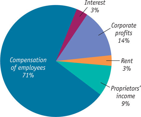
However, measured wages and benefits don’t capture the full income of “labor” because a significant fraction of total income in the United States (usually 7 to 10%) is “proprietors’ income”—the earnings of people who own their own businesses. Part of that income should be considered wages these business owners pay themselves. So the true share of labor in the economy is probably a few percentage points higher than the reported “compensation of employees” share.

But much of what we call compensation of employees is really a return on human capital. A surgeon isn’t just supplying the services of a pair of ordinary hands (at least the patient hopes not!): that individual is also supplying the result of many years and hundreds of thousands of dollars invested in training and experience. We can’t directly measure what fraction of wages is really a payment for education and training, but many economists believe that human capital has become the most important factor of production in modern economies.

Marginal Productivity and Factor Demand

All economic decisions are about comparing costs and benefits—and usually about comparing marginal costs and marginal benefits. This goes both for a consumer, deciding whether to buy more goods or services, and for a firm, deciding whether to hire an additional worker.

Although there are some important exceptions, most factor markets in the modern American economy are perfectly competitive. This means that most buyers and sellers of factors are price-takers because they are too small relative to the market to do anything but accept the market price. And in a competitive labor market, it’s clear how to define the marginal cost an employer pays for a worker: it is simply the worker’s wage rate. But what is the marginal benefit of that worker? To answer that question, we return to the production function, which relates inputs to output. For now we assume that all firms are price-takers in their output markets—that is, they operate in a perfectly competitive industry.

Value of the Marginal Product

Figure 40-2 reproduces Figures 21-1 and 21-2, which show the production function for wheat on George and Martha’s farm. Panel (a) of Figure 40-2 uses the total product curve to show how total wheat production depends on the number of workers employed on the farm; panel (b) shows how the marginal product of labor, the increase in output from employing one more worker, depends on the number of workers employed. Table 40-1 shows the numbers behind the figure. Note: sometimes the marginal product (MP) is called the marginal product of labor, or MPL.

Panel (a) shows how the quantity of output of wheat on George and Martha’s farm depends on the number of workers employed. Panel (b) shows how the marginal product of labor depends on the number of workers employed.

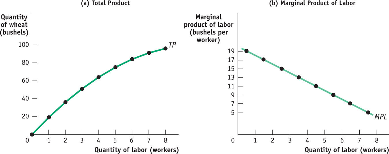
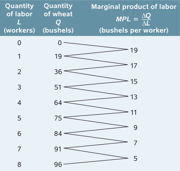
If workers are paid $200 each and wheat sells for $20 per bushel, how many workers should George and Martha employ to maximize profit?

Earlier we showed how to answer this question in several steps. First, we used information from the production function to derive the firm’s total cost and its marginal cost. Then we used the price-taking firm’s optimal output rule: a price-taking firm’s profit is maximized by producing the quantity of output at which the marginal cost is equal to the market price. Having determined the optimal quantity of output, we went back to the production function to find the optimal number of workers—which was simply the number of workers needed to produce the optimal quantity of output.

As you might have guessed, marginal analysis provides a more direct way to find the number of workers that maximizes a firm’s profit. This alternative approach is just a different way of looking at the same thing. But it gives us more insight into the demand for factors as opposed to the supply of goods.

To see how this alternative approach works, suppose that George and Martha are deciding whether to employ another worker. The increase in cost from employing another worker is the wage rate, W. The benefit to George and Martha from employing another worker is the value of the extra output that worker can produce. What is this value? It is the marginal product of labor, MPL, multiplied by the price per unit of output, P. This amount—the extra value of output generated by employing one more unit of labor—is known as the value of the marginal product of labor, or VMPL:

So should George and Martha hire another worker? Yes, if the value of the extra output is more than the cost of the additional worker—that is, if VMPL > W. Otherwise, they should not.

The hiring decision is made using marginal analysis, by comparing the marginal benefit from hiring another worker (VMPL) with the marginal cost (W). And as with any decision that is made on the margin, the optimal choice is made by equating marginal benefit with marginal cost (or if they’re never equal, by continuing to hire until the marginal cost of one more unit would exceed the marginal benefit). That is, to maximize profit, George and Martha will employ workers up to the point at which, for the last worker employed,

A firm should hire another worker if the value of the extra output is more than the cost of the additional worker.

Elena Elisseeva/ShutterstockA

This rule doesn’t apply only to labor; it applies to any factor of production. The value of the marginal product of any factor is its marginal product times the price of the good it produces. The general rule is that a profit-maximizing price-taking producer employs each factor of production up to the point at which the value of the marginal product of the last unit of the factor employed is equal to that factor’s price.

This rule is consistent with our previous analysis. We saw that a profit-maximizing firm chooses the level of output at which the price of the good it produces equals the marginal cost of producing that good. It turns out that if the level of output is chosen so that price equals marginal cost, then it is also true that with the amount of labor required to produce that output level, the value of the marginal product of labor will equal the wage rate.

Now let’s look more closely at why choosing the level of employment to equate VMPL and W works, and at how it helps us understand factor demand.

Value of the Marginal Product and Factor Demand

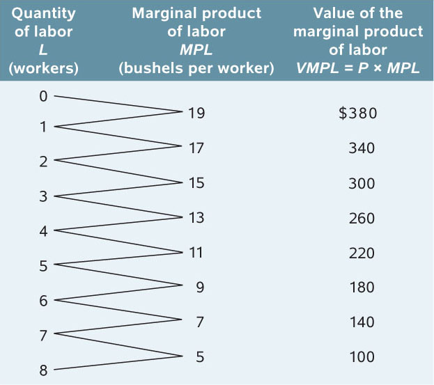
Table 40-2 shows the value of the marginal product of labor on George and Martha’s farm when the price of wheat is $20 per bushel. In Figure 40-3, the horizontal axis shows the number of workers employed; the vertical axis measures the value of the marginal product of labor and the wage rate. The curve shown is the value of the marginal product curve of labor. This curve, like the marginal product of labor curve, slopes downward because of diminishing returns to labor in production. That is, the value of the marginal product of each worker is less than that of the preceding worker because the marginal product of each worker is less than that of the preceding worker.

This curve shows how the value of the marginal product of labor depends on the number of workers employed. It slopes downward because of diminishing returns to labor in production. To maximize profit, George and Martha choose the level of employment at which the value of the marginal product of labor is equal to the market wage rate. For example, at a wage rate of $200 the profit-maximizing level of employment is 5 workers, shown by point A. 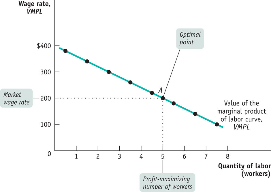The value of the marginal product curve of a factor is the producer’s individual demand curve for that factor.

We have just seen that to maximize profit, George and Martha hire workers until the wage rate is equal to the value of the marginal product of the last worker employed. Let’s use the example to see how this principle really works. Assume that George and Martha currently employ 3 workers and that these workers must be paid the market wage rate of $200. Should they employ an additional worker?

Looking at Table 40-2, we see that if George and Martha currently employ 3 workers, the value of the marginal product of an additional worker is $260. So if they employ an additional worker, they will increase the value of their production by $260 but increase their cost by only $200, yielding an increased profit of $60. In fact, a firm can always increase profit by employing one more unit of a factor of production as long as the value of the marginal product produced by that unit exceeds the factor price.

Alternatively, suppose that George and Martha employ 8 workers. By reducing the number of workers to 7, they can save $200 in wages. In addition, the value of the marginal product of the 8th worker is only $100. So, by reducing employment by one worker, they can increase profit by $200 − $100 = $100. In other words, a firm can always increase profit by employing one less unit of a factor of production as long as the value of the marginal product produced by that unit is less than the factor price.

Using this method, we can see from Table 40-2 that the profit-maximizing employment level is 5 workers, given a wage rate of $200. The value of the marginal product of the 5th worker is $220, so adding the 5th worker results in $20 of additional profit.

But George and Martha should not hire more than 5 workers: the value of the marginal product of the 6th worker is only $180, $20 less than the cost of that worker. So, to maximize profit, George and Martha should employ workers up to but not beyond the point at which the value of the marginal product of the last worker employed is equal to the wage rate.

Firms keep hiring more workers until the value of the marginal product of labor equals the wage rate.

© Ilene MacDonald/AlamyReview

Now look again at the value of the marginal product curve in Figure 40-3. To determine the profit-maximizing level of employment, we set the value of the marginal product of labor equal to the price of labor—a wage rate of $200 per worker. This means that the profit-maximizing level of employment is at point A, corresponding to an employment level of 5 workers. If the wage rate were higher, we would simply move up the curve and decrease the number of workers employed: if the wage rate were lower than $200, we would move down the curve and increase the number of workers employed.

In this example, George and Martha have a small farm in which the potential employment level varies from 0 to 8 workers, and they hire workers up to the point at which the value of the marginal product of another worker would fall below the wage rate.

For a larger farm with many employees, the value of the marginal product of labor falls only slightly when an additional worker is employed. As a result, there will be some worker whose value of the marginal product almost exactly equals the wage rate. (In keeping with the George and Martha example, this means that some worker generates a value of the marginal product of approximately $200.) In this case, the firm maximizes profit by choosing a level of employment at which the value of the marginal product of the last worker hired equals (to a very good approximation) the wage rate.

In the interest of simplicity, we will assume from now on that firms use this rule to determine the profit-maximizing level of employment. This means that the value of the marginal product of labor curve is the individual firm’s labor demand curve. And in general, a firm’s value of the marginal product curve for any factor of production is that firm’s individual demand curve for that factor of production.

Shifts of the Factor Demand Curve

As in the case of ordinary demand curves, it is important to distinguish between movements along the factor demand curve and shifts of the factor demand curve. What causes factor demand curves to shift? There are three main causes:

1. Changes in the prices of goods
2. Changes in the supply of other factors
3. Changes in technology

1. Changes in the Prices of GoodsRemember that factor demand is derived demand: if the price of the good that is produced with a factor changes, so will the value of the marginal product of the factor. That is, in the case of labor demand, if P changes, VMPL = P × MPL will change at any given level of employment.

Figure 40-4 illustrates the effects of changes in the price of wheat, assuming that $200 is the current wage rate. Panel (a) shows the effect of an increase in the price of wheat. This shifts the value of the marginal product of labor curve upward because VMPL rises at any given level of employment. If the wage rate remains unchanged at $200, the optimal point moves from point A to point B: the profit-maximizing level of employment rises.

Panel (a) shows the effect of an increase in the price of wheat on George and Martha’s demand for labor. The value of the marginal product of labor curve shifts upward, from VMPL₁ to VMPL₂. If the market wage rate remains at $200, profit-maximizing employment rises from 5 workers to 8 workers, shown by the movement from point A to point B. Panel (b) shows the effect of a decrease in the price of wheat. The value of the marginal product of labor curve shifts downward, from VMPL₁ to VMPL₃. At the market wage rate of $200, profit-maximizing employment falls from 5 workers to 2 workers, shown by the movement from point A to point C.

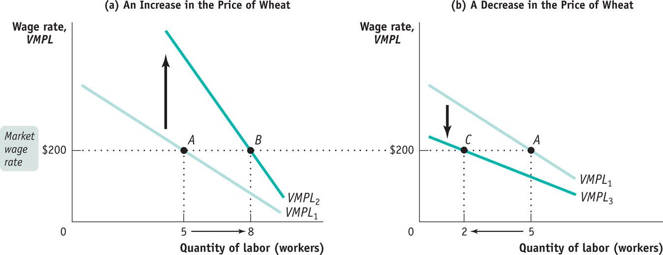
Panel (b) shows the effect of a decrease in the price of wheat. This shifts the value of the marginal product of labor curve downward. If the wage rate remains unchanged at $200, the optimal point moves from point A to point C: the profit-maximizing level of employment falls.

2. Changes in the Supply of Other FactorsSuppose that George and Martha acquire more land to cultivate—say, by clearing a woodland on their property. Each worker now produces more wheat because each one has more land to work with. As a result, the marginal product of labor on the farm rises at any given level of employment. This has the same effect as an increase in the price of wheat, which is illustrated in panel (a) of Figure 40-4: the value of the marginal product of labor curve shifts upward, and at any given wage rate the profit-maximizing level of employment rises. Similarly, suppose George and Martha cultivate less land. This leads to a fall in the marginal product of labor at any given employment level. Each worker produces less wheat because each has less land to work with. As a result, the value of the marginal product of labor curve shifts downward—as in panel (b) of Figure 40-4—and the profit-maximizing level of employment falls.

3. Changes in TechnologyIn general, the effect of technological progress on the demand for any given factor can go either way: improved technology can either increase or decrease the demand for a given factor of production.

How can technological progress decrease factor demand? Consider horses, which were once an important factor of production. The development of substitutes for horse power, such as automobiles and tractors, greatly reduced the demand for horses.

The usual effect of technological progress, however, is to increase the demand for a given factor, often because it raises the marginal product of the factor. In particular, although there have been persistent fears that machinery would reduce the demand for labor, over the long run the U.S. economy has seen both large wage increases and large increases in employment, suggesting that technological progress has greatly increased labor demand.

Module 40 Review

Check Your Understanding

Draw three separate, correctly labeled graphs illustrating the effect of each of the following changes on the demand for labor. Adopt the usual ceteris paribus assumption that all else remains unchanged in each case.

• a. The price of the product being produced decreases.
• b. Worker productivity increases.
• c. Firms invest in more capital to be used by workers.

PITFALLS: WHAT IS A FACTOR, ANYWAY?

WHAT IS A FACTOR, ANYWAY?

Imagine a business that produces shirts. The business will make use of workers and machines—that is, of labor and capital. But it will also use other inputs, such as electricity and cloth. Are all of these inputs factors of production?

No: labor and physical capital are factors of production, but cloth and electricity are not. The key distinction is that a factor of production earns income from the selling of its services over and over again but an input cannot. For example, a worker earns income over time from repeatedly selling his or her efforts; the owner of a machine earns income over time from repeatedly selling the use of that machine. So a factor of production, such as labor and physical capital, represents an enduring source of income. An input like electricity or cloth, however, is used up in the production process. Once exhausted, it cannot be a source of future income for its owner.

To learn more, see the discussion on pages 424–425.