1.3 Module 26: Graphing Perfect Competition

iStockphoto

In the previous module we learned how to compare market price and average total cost to determine whether or not a competitive firm is profitable. Now we can evaluate the profitability of perfectly competitive firms in a variety of situations.

Interpreting Perfect Competition Graphs

Figure 26-1 illustrates how the market price determines whether a firm is profitable. It also shows how profits are depicted graphically. Each panel shows the marginal cost curve, MC, and the short-run average total cost curve, ATC. Average total cost is minimized at point C. Panel (a) shows the case in which the market price of tomatoes is $18 per bushel. Panel (b) shows the case in which the market price of tomatoes is lower, $10 per bushel.

In panel (a) the market price is $18. The farm is profitable because price exceeds minimum average total cost, the break-even price, $14. The farm’s optimal output choice is indicated by point E, corresponding to an output of 5 bushels. The average total cost of producing 5 bushels is indicated by point Z on the ATC curve, corresponding to an amount of $14.40. The vertical distance between E and Z corresponds to the farm’s per-unit profit, $18.00 − $14.40 = $3.60. Total profit is given by the area of the shaded rectangle, 5 × $3.60 = $18.00. In panel (b) the market price is $10; the farm is unprofitable because the price falls below the minimum average total cost, $14. The farm’s optimal output choice when producing is indicated by point A, corresponding to an output of 3 bushels. The farm’s per-unit loss, $14.67 − $10.00 = $4.67, is represented by the vertical distance between A and Y. The farm’s total loss is represented by the shaded rectangle, 3 × $4.67 = $14.00 (adjusted for rounding error).

In panel (a), we see that at a price of $18 per bushel the profit-maximizing quantity of output is 5 bushels, indicated by point E, where the marginal cost curve, MC, intersects the marginal revenue curve, MR—which for a price-taking firm is a horizontal line at the market price. At that quantity of output, average total cost is $14.40 per bushel, indicated by point Z. Since the price per bushel exceeds the average total cost per bushel, Jennifer and Jason’s farm is profitable.

Jennifer and Jason’s total profit when the market price is $18 is represented by the area of the shaded rectangle in panel (a). To see why, notice that total profit can be expressed in terms of profit per unit:

or, equivalently, because P is equal to TR/Q and ATC is equal to TC/Q,

The height of the shaded rectangle in panel (a) corresponds to the vertical distance between points E and Z. It is equal to P − ATC = $18.00 − $14.40 = $3.60 per bushel. The shaded rectangle has a width equal to the output: Q = 5 bushels. So the area of that rectangle is equal to Jennifer and Jason’s profit: 5 bushels × $3.60 profit per bushel = $18.

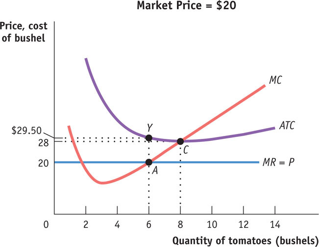
What about the situation illustrated in panel (b)? Here the market price of tomatoes is $10 per bushel. Producing until price equals marginal cost leads to a profit-maximizing output of 3 bushels, indicated by point A. At this output, Jennifer and Jason have an average total cost of $14.67 per bushel, indicated by point Y. At their profit-maximizing output quantity—3 bushels—average total cost exceeds the market price. This means that Jennifer and Jason’s farm generates a loss, not a profit.

How much do they lose by producing when the market price is $10? On each bushel they lose ATC − P = $14.67 − $10.00 = $4.67, an amount corresponding to the vertical distance between points A and Y. And they produce 3 bushels, which corresponds to the width of the shaded rectangle. So the total value of the losses is $4.67 × 3 = $14.00 (adjusted for rounding error), an amount that corresponds to the area of the shaded rectangle in panel (b).

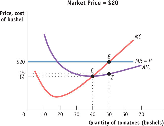
But how does a producer know, in general, whether or not its business will be profitable? It turns out that the crucial test lies in a comparison of the market price to the firm’s minimum average total cost. On Jennifer and Jason’s farm, average total cost reaches its minimum, $14, at an output of 4 bushels, indicated by point C. Whenever the market price exceeds the minimum average total cost, there are output levels for which the average total cost is less than the market price. In other words, the producer can find a level of output at which the firm makes a profit. So Jennifer and Jason’s farm will be profitable whenever the market price exceeds $14. And they will achieve the highest possible profit by producing the quantity at which marginal cost equals price.

A firm will earn positive profit when the market price is above the break-even price.

Thinkstock

Conversely, if the market price is less than the minimum average total cost, there is no output level at which price exceeds average total cost. As a result, the firm will be unprofitable at any quantity of output. As we saw, at a price of $10—an amount less than the minimum average total cost—Jennifer and Jason did indeed lose money. By producing the quantity at which marginal cost equaled price, Jennifer and Jason did the best they could, but the best they could do was a loss of $14. Any other quantity would have increased the size of their loss.

The minimum average total cost of a price-taking firm is called its break-even price, the market price at which it earns zero economic profit.A firm will earn positive profit when the market price is above the break-even price, and it will suffer losses when the market price is below the break-even price. Jennifer and Jason’s break-even price of $14 is the price at point C in Figure 26-1.

So the rule for determining whether a firm is profitable depends on a comparison of the market price of the good to the firm’s break-even price—its minimum average total cost:

• Whenever the market price exceeds the minimum average total cost, the producer is profitable.
• Whenever the market price equals the minimum average total cost, the producer breaks even.
• Whenever the market price is less than the minimum average total cost, the producer is unprofitable.

The Short-Run Production Decision

You might be tempted to say that if a firm is unprofitable because the market price is below its minimum average total cost, it shouldn’t produce any output. In the short run, however, this conclusion isn’t right. In the short run, sometimes the firm should produce even if price falls below minimum average total cost. The reason is that total cost includes fixed cost—cost that does not depend on the amount of output produced and can be altered only in the long run. In the short run, fixed cost must still be paid, regardless of whether or not a firm produces. For example, if Jennifer and Jason have rented a tractor for the year, they have to pay the rent on the tractor regardless of whether they produce any tomatoes. Since it cannot be changed in the short run, their fixed cost is irrelevant to their decision about whether to produce or shut down in the short run.

Although fixed cost should play no role in the decision about whether to produce in the short run, another type of cost—variable cost—does matter. Part of the variable cost for Jennifer and Jason is the wage cost of workers who must be hired to help with planting and harvesting. Variable cost can be eliminated by not producing, which makes it a critical consideration when determining whether or not to produce in the short run.

Let’s turn to Figure 26-2: it shows both the short-run average total cost curve, ATC, and the short-run average variable cost curve, AVC, drawn from the information in Table 25-3. Recall that the difference between the two curves—the vertical distance between them—represents average fixed cost, the fixed cost per unit of output, FC/Q. Because the marginal cost curve has a “swoosh” shape—falling at first before rising—the short-run average variable cost curve is U-shaped: the initial fall in marginal cost causes average variable cost to fall as well, and then the rise in marginal cost eventually pulls average variable cost up again. The short-run average variable cost curve reaches its minimum value of $10 at point A, at an output of 3 bushels.

When the market price equals or exceeds Jennifer and Jason’s shut-down price of $10, the minimum average variable cost indicated by point A, they will produce the output quantity at which marginal cost is equal to price. So at any price equal to or above the minimum average variable cost, the short-run individual supply curve is the firm’s marginal cost curve; this corresponds to the upward-sloping segment of the individual supply curve. When market price falls below minimum average variable cost, the firm ceases operation in the short run. This corresponds to the vertical segment of the individual supply curve along the vertical axis.

The Shut-Down Price

We are now prepared to analyze the optimal production decision in the short run. We have two cases to consider:

• When the market price is below the minimum average variable cost
• When the market price is greater than or equal to the minimum average variable cost

When the market price is below the minimum average variable cost, the price the firm receives per unit is not covering its variable cost per unit. A firm in this situation should cease production immediately. Why? Because there is no level of output at which the firm’s total revenue covers its variable cost—the cost it can avoid by not operating. In this case the firm maximizes its profit by not producing at all—by, in effect, minimizing its loss. It will still incur a fixed cost in the short run, but it will no longer incur any variable cost. This means that the minimum average variable cost determines the shut-down price, the price at which the firm ceases production in the short run.

When price is greater than minimum average variable cost, however, the firm should produce in the short run. In this case, the firm maximizes profit—or minimizes loss—by choosing the output level at which its marginal cost is equal to the market price. For example, if the market price of tomatoes is $18 per bushel, Jennifer and Jason should produce at point E in Figure 26-2, corresponding to an output of 5 bushels. Note that point C in Figure 26-2 corresponds to the farm’s break-even price of $14 per bushel. Since E lies above C, Jennifer and Jason’s farm will be profitable; they will generate a per-bushel profit of $18.00 − $14.40 = $3.60 when the market price is $18.

But what if the market price lies between the shut-down price and the break-even price—that is, between the minimum average variable cost and the minimum average total cost? In the case of Jennifer and Jason’s farm, this corresponds to prices anywhere between $10 and $14—say, a market price of $12. At $12, Jennifer and Jason’s farm is not profitable; since the market price is below the minimum average total cost, the farm is losing (on average) the difference between price and average total cost on every unit produced. Yet even though the market price isn’t covering Jennifer and Jason’s average total cost, it is covering their average variable cost and some—but not all—of the average fixed cost. If a firm in this situation shuts down, it will incur no variable cost but it will incur the full fixed cost. As a result, shutting down will generate an even greater loss than continuing to operate.

In the short-run production decision, a firm’s fixed cost is essentially a sunk cost

Anthony Masterson/Digital Vision/Getty Images

This means that whenever price falls between minimum average total cost and minimum average variable cost, the firm is better off producing some output in the short run. The reason is that by producing, it can cover its variable cost and at least some of its fixed cost, even though it is incurring a loss. In this case, the firm maximizes profit—that is, minimizes loss—by choosing the quantity of output at which its marginal cost is equal to the market price. So if Jennifer and Jason face a market price of $12 per bushel, their profit-maximizing output is given by point B in Figure 26-2, corresponding to an output of 3.5 bushels.

It’s worth noting that the decision to produce when the firm is covering its variable cost but not all of its fixed cost is similar to the decision to ignore a sunk cost, a concept we studied previously. You may recall that a sunk cost is a cost that has already been incurred and cannot be recouped; and because it cannot be changed, it should have no effect on any current decision. In the short-run production decision, fixed cost is, in effect, like a sunk cost—it has been spent, and it can’t be recovered in the short run. This comparison also illustrates why variable cost does indeed matter in the short run: it can be avoided by not producing.

And what happens if the market price is exactly equal to the shut-down price, the minimum average variable cost? In this instance, the firm is indifferent between producing 3 units or 0 units. As we’ll see shortly, this is an important point when looking at the behavior of an industry as a whole. For the sake of clarity, we’ll assume that the firm, although indifferent, does indeed produce output when price is equal to the shut-down price.

Putting everything together, we can now draw the short-run individual supply curve of Jennifer and Jason’s farm, the red line in Figure 26-2; it shows how the profit--maximizing quantity of output in the short run depends on the price. As you can see, the curve is in two segments. The upward-sloping red segment starting at point A shows the short-run profit-maximizing output when market price is equal to or above the shut-down price of $10 per bushel.

Some firms shut down temporarily without going out of business.

V.e.r.i.k/Dreamstime.com

As long as the market price is equal to or above the shut-down price, Jennifer and Jason will produce the quantity of output at which marginal cost is equal to the market price. So at market prices equal to or above the shut-down price, the firm’s short-run supply curve corresponds to its marginal cost curve. But at any market price below the minimum average variable cost, in this case, $10 per bushel—the firm shuts down and output drops to zero in the short run. This corresponds to the vertical segment of the curve that lies on top of the vertical axis.

Do firms sometimes shut down temporarily without going out of business? Yes. In fact, in some industries temporary shut-downs are routine. The most common examples are industries in which demand is highly seasonal, like outdoor amusement parks in climates with cold winters. Such parks would have to offer very low prices to entice customers during the colder months—prices so low that the owners would not cover their variable cost (principally wages and electricity). The wiser choice economically is to shut down until warm weather brings enough customers who are willing to pay a higher price.

Changing Fixed Cost

Although fixed cost cannot be altered in the short run, in the long run firms can acquire or get rid of machines, buildings, and so on. In the long run the level of fixed cost is a matter of choice, and a firm will choose the level of fixed cost that minimizes the average total cost for its desired output level. Now we will focus on an even bigger question facing a firm when choosing its fixed cost: whether to incur any fixed cost at all by continuing to operate.

In the long run, a firm can always eliminate fixed cost by selling off its plant and equipment. If it does so, of course, it can’t produce any output—it has exited the industry. In contrast, a new firm can take on some fixed cost by acquiring machines and other resources, which puts it in a position to produce—it can enter the industry. In most perfectly competitive industries the set of firms, although fixed in the short run, changes in the long run as some firms enter or exit the industry.

Consider Jennifer and Jason’s farm once again. In order to simplify our analysis, we will sidestep the issue of choosing among several possible levels of fixed cost. Instead, we will assume that if they operate at all, Jennifer and Jason have only one possible choice of fixed cost: $14. Alternatively, they can choose a fixed cost of zero if they exit the industry. It is changes in fixed cost that cause short-run average total cost curves to differ from long-run average total cost curves, so with this assumption, Jennifer and Jason’s short-run and long-run average total cost curves are one and the same.

Suppose that the market price of organic tomatoes is consistently less than the break-even price of $14 over an extended period of time. In that case, Jennifer and Jason never fully cover their total cost: their business runs at a persistent loss. In the long run, then, they can do better by closing their business and leaving the industry. In other words, in the long run firms will exit an industry if the market price is consistently less than their break-even price—their minimum average total cost.

Conversely, suppose that the price of organic tomatoes is consistently above the break-even price, $14, for an extended period of time. Because their farm is profitable, Jennifer and Jason will remain in the industry and continue producing.

But things won’t stop there. The organic tomato industry meets the criterion of free entry: there are many potential organic tomato producers because the necessary inputs are easy to obtain. And the cost curves of those potential producers are likely to be similar to those of Jennifer and Jason, since the technology used by other producers is likely to be very similar to that used by Jennifer and Jason. If the price is high enough to generate profits for existing producers, it will also attract some of these potential producers into the industry. So in the long run a price in excess of $14 should lead to entry: new producers will come into the organic tomato industry.

As we will see shortly, exit and entry lead to an important distinction between the short-run industry supply curve and the long-run industry supply curve.

PRICES ARE UP … BUT SO ARE COSTS

Because of the Energy Policy Act of 2005, 7.5 billion gallons of alternative fuel, mostly corn-based ethanol, was added to the American fuel supply to help reduce gasoline consumption. The unsurprising result of this mandate: the demand for corn skyrocketed, along with its price. In August 2012, a bushel of corn hit a high of $8.32, nearly quadruple the January 2005 price of $2.09.

This sharp rise in the price of corn caught the eye of American farmers like Ronnie Gerik of Aquilla, Texas, who, in response to surging corn prices, reduced the size of his cotton crop and increased his corn acreage by 40%. He was not alone; overall, the U.S. corn acreage planted in 2011 was 9% more than the average planted over the previous decade. And 4% more was planted in 2012.

Although Gerik was taking a big gamble when he cut the size of his cotton crop to plant more corn, his decision made good economic sense.

Courtesy of Ronnie Gerik.

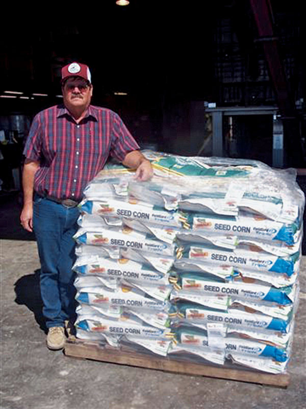
Although this sounds like a sure way to make a profit, Gerik was actually taking a big gamble: even though the price of corn increased, so did the cost of the raw materials needed to grow it—by 20%. Consider the cost of just two inputs: fertilizer and fuel. Corn requires more fertilizer than other crops and, with more farmers planting corn, the increased demand for fertilizer led to a price increase.

Moreover, corn is much more sensitive to the amount of rainfall than a crop like cotton. So farmers who plant corn in drought-prone places like Texas are increasing their risk of loss. Gerik had to incorporate into his calculations his best guess of what a dry spell would cost him.

Despite all of this, what Gerik did made complete economic sense. By planting more corn, he was moving up his individual short-run supply curve for corn production. And because his individual supply curve is his marginal cost curve, his costs also went up because he had to use more inputs—inputs that had become more expensive to obtain.

So the moral of this story is that farmers will increase their corn acreage until the marginal cost of producing corn is approximately equal to the market price of corn—which shouldn’t come as a surprise because corn production satisfies all the requirements of a perfectly competitive industry.

Summing Up: The Perfectly Competitive Firm’s Profitability and Production Conditions

In this module we’ve studied what’s behind the supply curve for a perfectly competitive, price-taking firm. A perfectly competitive firm maximizes profit, or minimizes loss, by producing the quantity that equates price and marginal cost. The exception is if price is below minimum average variable cost in the short run, or below minimum average total cost in the long run, in which case the firm is better off shutting down. Table 26-1 summarizes the perfectly competitive firm’s profitability and production conditions. It also relates them to entry into and exit from the industry in the long run. Now that we understand how a perfectly competitive firm makes its decisions, we can go on to look at the supply curve for a perfectly competitive market and the long-run market equilibrium in perfect competition.

Module 26 Review

Check Your Understanding

To answer questions 1–3, refer to the graph provided.

Question

ahB7p+4s+GzFOS7X1u22xy7Lg/3vSh4ZMaoy1QWsTTau0UMfCWCidVPxU/jonAg8mZMw3eRN+Hisb9qOBLFB0KpQloXGZbCeMhT4t/qzc7d0DqduPkB5WUTzuQc8CeBPlbpRPEHdkDQ+gn1KBw+knyQtM9x4WezjmsPEdoFQURNyUAjZ/hxmLiBBtZ+IqCrTY4nPcos18SIgN/X46KCxxw==

Question

US4zMCPckxm16qvWwTkFmMcFzkokhYRa990d2Z7AlkuXMZhEFnaLi77gXAZ6x3pjcdl0eEU6686MplqRrjdOyM9BIDbckvVtUV5ckM/fsPfcSNoaEAoOvsfdHh1LY968d9IlBHYXqBin3B6zeXTX1/91tccCamQv9sxw/3kxwlwN9UGpNfx4okrjt1ZuOL0SNXXKhJlfUsPrPVqd

Question

BW5hVp/EjiJI11nlWn/2hC8gN1gE2lnnSfFyH59FHEyq3gcPBWMtQUYykofpquxIXM/4FzHaI7alvm+rv5QvNdi/TCqmVpLqIyLFuPa7Id+OIsa26V/HrkGocaHMw1KpU1w61nVsVVG0J+BSRg14IfRtG9axasVJoQp3PzOJRKns+9Az3l6jwnw9EPPvZeYKXmPKCcWdeVztK3uRdFlHh7AO+1A0NpRnsOq0FbXtFZj21e48FUlEIP4WjTTfprIVSSFggMlpmeV2DU/E4nI0MXfMXRc=

Question

bzxVP1ZSS66PbTN1lK9UCpnUk70T44cQs6LLBDl+WMZ0rr27kwILP0mp8UtVCAzyMC8cZIq17WjP2X0VQq7TujmmXvREiBrUVO8VjnC3gub02UB+xDamRyxtZDg1EFWPC77J5mwtvDz9SMWcCyJbnjynBGM3h3ItdIpbKGkw2WzDpa59GEMzyexUNayqU8wwo7leDSHGPGakF5+Brs9s70mYtR7lHldZvqidU220yNYSm0k1TmDQd9hDo0SlAV3eYgLS8XDicGsPmWXnYGa5T0wdFYodiXyd94KWFw70RxmC/n+jtbJ3cCKm4NAQbCi6BUBPCm9zk8nmMlMWNTnpPd3SU8Onw5de

Question

LVl9JfgzvCEvmFYv9iixPzXy7q2/J3/QgvMLUiFGsOPb53c88lo5Fo2OkGZr1ULncywQJgwAo90KqfqLXmdCVFNc85CNeK1D0FoiSOKVngtKWL615QPJaX2P85njM1b6biucWLa+6hA5DoE9rczdOJeyNWsaOHHzBnvhU+i4kLWHzcY5nW6h6AVUAyRNtQRO84Y4Gg6UDhSHboI11MfI5usAL9lgIfy3RFD+aLBvzZSnS3bgKKjB1CYFSwjBgW4FFJWijKR0lK7nZpnxtxp/bMX84mdYgYz9hOsdkGyNinucOB5IxfTpzR9T8Mdawfj3NkMOnBdIoVKdk2tex1mkMOou055wN5G2ctu3jZhpQ/fiETcKV0IC2fHefr1iY331kNI3AXhrQFbNu0qxB2qQ62/4blgCGmt83Itj2eNKCMxECztJiJTCDJtMXzoSPxyFzo8vDSWQbXHQtTI8TlEgPrUTGir2XEjKDf7Gr7rYq1obzTBb0wwa+y3zqq4=

Refer to the graph provided to answer the questions that follow.