Summing Up: The Perfectly Competitive Firm’s Profitability and Production Conditions
In this chapter, we’ve studied where the supply curve for a perfectly competitive, price-
|
Profitability condition (minimum ATC = break- |
Result |
|
P > minimum ATC |
Firm profitable. Entry into industry in the long run. |
|
P = minimum ATC |
Firm breaks even. No entry into or exit from industry in the long run. |
|
P < minimum ATC |
Firm unprofitable. Exit from industry in the long run. |
|
Production condition (minimum AVC = shut- |
Result |
|
P > minimum AVC |
Firm produces in the short run. If P < minimum ATC, firm covers variable cost and some but not all of fixed cost. If P > minimum ATC, firm covers all variable cost and fixed cost. |
|
P = minimum AVC |
Firm indifferent between producing in the short run or not. Just covers variable cost. |
|
P < minimum AVC |
Firm shuts down in the short run. Does not cover variable cost. |
TABLE 12-
!worldview! ECONOMICS in Action: Farmers Move Up Their Supply Curves
Farmers Move Up Their Supply Curves

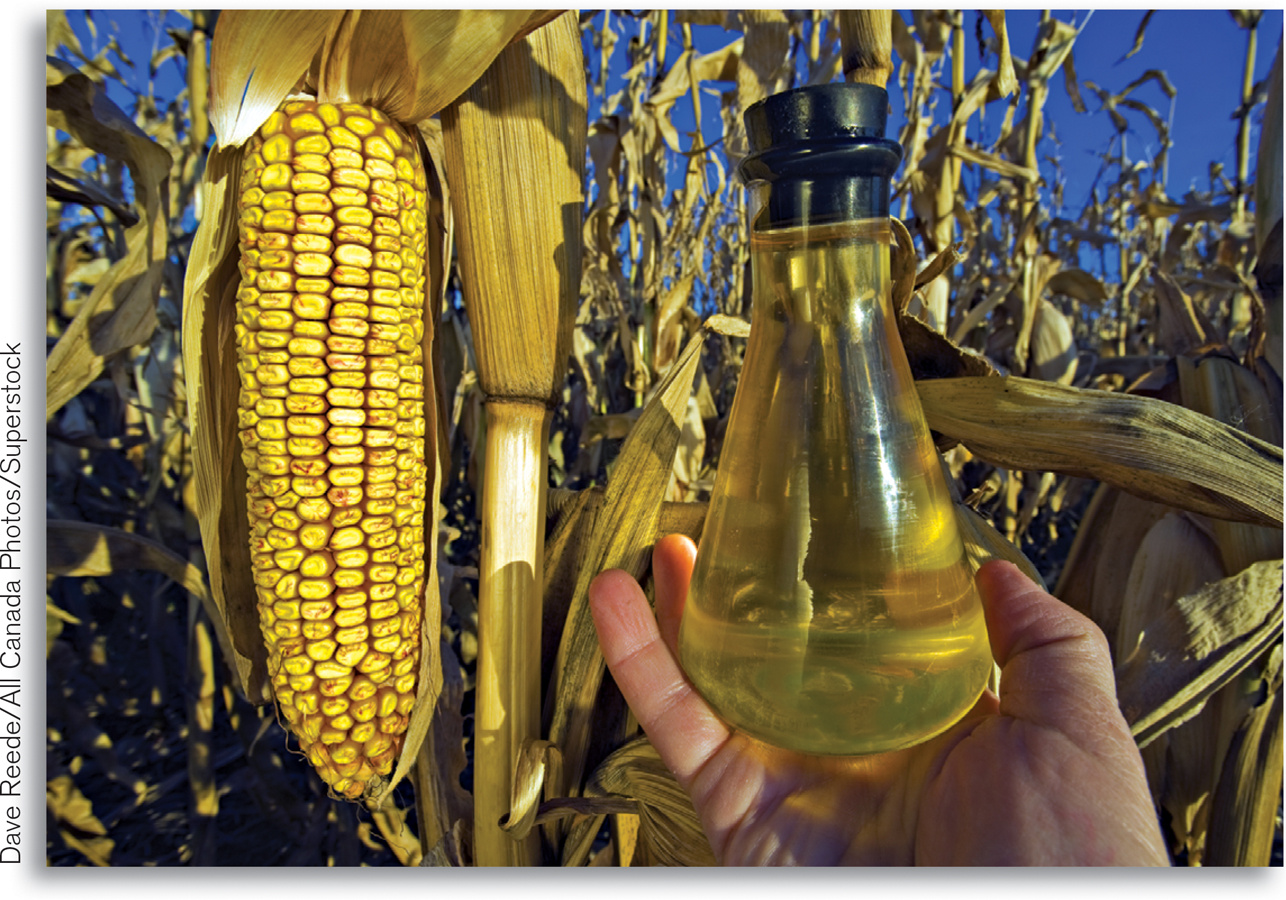
To reduce gasoline consumption, Congress mandated that increasing amounts of biofuel, mostly corn-
If this sounds like a sure way to make a profit, think again. Corn farmers were taking a considerable gamble in planting more corn as their costs went up. Consider the cost of fertilizer, an important input. Corn requires more fertilizer than other crops, and with more farmers planting corn, the increased demand for fertilizer led to a price increase. In 2006 and 2007, fertilizer prices surged to five times their 2005 level; by 2013 prices were still twice as high.
The pull of higher corn prices also lifted farmland prices to record levels—
Despite the risk and increase in costs, what corn farmers did made complete economic sense. By planting more corn, each farmer moved up his or her individual supply curve. And because the individual supply curve is the marginal cost curve, each farmer’s costs also went up because of the need to use more inputs that are now more expensive to obtain.
So the moral of the story is that farmers will increase their corn acreage until the marginal cost of producing corn is approximately equal to the market price of corn—
Quick Review
A producer chooses output according to the optimal output rule. For a price-
taking firm, marginal revenue is equal to price and it chooses output according to the price- taking firm’s optimal output rule P = MC. A firm is profitable whenever price exceeds its break-
even price, equal to its minimum average total cost. Below that price it is unprofitable. It breaks even when price is equal to its break- even price. Fixed cost is irrelevant to the firm’s optimal short-
run production decision. When price exceeds its shut- down price, minimum average variable cost, the price- taking firm produces the quantity of output at which marginal cost equals price. When price is lower than its shut- down price, it ceases production in the short run. This defines the firm’s short- run individual supply curve. Over time, fixed cost matters. If price consistently falls below minimum average total cost, a firm will exit the industry. If price exceeds minimum average total cost, the firm is profitable and will remain in the industry; other firms will enter the industry in the long run.
12-2
Question 12.2
Draw a short-
run diagram showing a U- shaped average total cost curve, a U- shaped average variable cost curve, and a “swoosh”-shaped marginal cost curve. On it, indicate the range of output and the range of price for which the following actions are optimal. The firm shuts down immediately.
The firm operates in the short run despite sustaining a loss.
The firm operates while making a profit.
Question 12.3
The state of Maine has a very active lobster industry, which harvests lobsters during the summer months. During the rest of the year, lobsters can be obtained from other parts of the world but at a much higher price. Maine is also full of “lobster shacks,” roadside restaurants serving lobster dishes that are open only during the summer. Explain why it is optimal for lobster shacks to operate only during the summer.
Solutions appear at back of book.