Using Marginal Analysis to Choose the Profit-Maximizing Quantity of Output
Marginal revenue is the change in total revenue generated by an additional unit of output.
Recall from Chapter 9 the profit-maximizing principle of marginal analysis: the optimal amount of an activity is the level at which marginal benefit is equal to marginal cost. To apply this principle, consider the effect on a producer’s profit of increasing output by one unit. The marginal benefit of that unit is the additional revenue generated by selling it; this measure has a name—it is called the marginal revenue of that unit of output. The general formula for marginal revenue is:
According to the optimal output rule, profit is maximized by producing the quantity of output at which the marginal revenue of the last unit produced is equal to its marginal cost.
So Noelle maximizes her profit by producing trees up to the point at which the marginal revenue is equal to marginal cost. We can summarize this as the producer’s optimal output rule: profit is maximized by producing the quantity at which the marginal revenue of the last unit produced is equal to its marginal cost. That is, MR = MC at the optimal quantity of output.
We can learn how to apply the optimal output rule with the help of Table 12-2, which provides various short-run cost measures for Noelle’s farm. The second column contains the farm’s variable cost, and the third column shows its total cost of output based on the assumption that the farm incurs a fixed cost of $140. The fourth column shows marginal cost. Notice that, in this example, the marginal cost initially falls as output rises but then begins to increase. This gives the marginal cost curve the “swoosh” shape described in the Selena’s Gourmet Salsas example in Chapter 11. Shortly it will become clear that this shape has important implications for short-run production decisions.
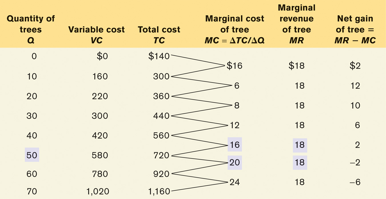
TABLE 12-2 Short-Run Costs for Noelle’s Farm
The fifth column contains the farm’s marginal revenue, which has an important feature: Noelle’s marginal revenue equal to price is constant at $18 for every output level. The sixth and final column shows the calculation of the net gain per tree, which is equal to marginal revenue minus marginal cost—or, equivalently in this case, market price minus marginal cost. As you can see, it is positive for the 10th through 50th trees; producing each of these trees raises Noelle’s profit. For the 60th through 70th trees, however, net gain is negative: producing them would decrease, not increase, profit. (You can verify this by examining Table 12-1.) So a quantity of 50 trees is Noelle’s profit-maximizing output; it is the level of output at which marginal cost is equal to the market price, $18.
According to the price-taking firm’s optimal output rule, a price-taking firm’s profit is maximized by producing the quantity of output at which the market price is equal to the marginal cost of the last unit produced.
This example, in fact, illustrates another general rule derived from marginal analysis—the price-taking firm’s optimal output rule, which says that a price-taking firm’s profit is maximized by producing the quantity of output at which the market price is equal to the marginal cost of the last unit produced. That is, P = MC at the price-taking firm’s optimal quantity of output. In fact, the price-taking firm’s optimal output rule is just an application of the optimal output rule to the particular case of a price-taking firm. Why? Because in the case of a price-taking firm, marginal revenue is equal to the market price.
A price-taking firm cannot influence the market price by its actions. It always takes the market price as given because it cannot lower the market price by selling more or raise the market price by selling less. So, for a price-taking firm, the additional revenue generated by producing one more unit is always the market price. We will need to keep this fact in mind in future chapters, where we will learn that marginal revenue is not equal to the market price if the industry is not perfectly competitive. As a result, firms are not price-takers when an industry is not perfectly competitive.
The marginal revenue curve shows how marginal revenue varies as output varies.
For the remainder of this chapter, we will assume that the industry in question is like Christmas tree farming, perfectly competitive. Figure 12-1 shows that Noelle’s profit-maximizing quantity of output is, indeed, the number of trees at which the marginal cost of production is equal to price. The figure shows the marginal cost curve, MC, drawn from the data in the fourth column of Table 12-2. As in Chapter 9, we plot the marginal cost of increasing output from 10 to 20 trees halfway between 10 and 20, and so on. The horizontal line at $18 is Noelle’s marginal revenue curve.
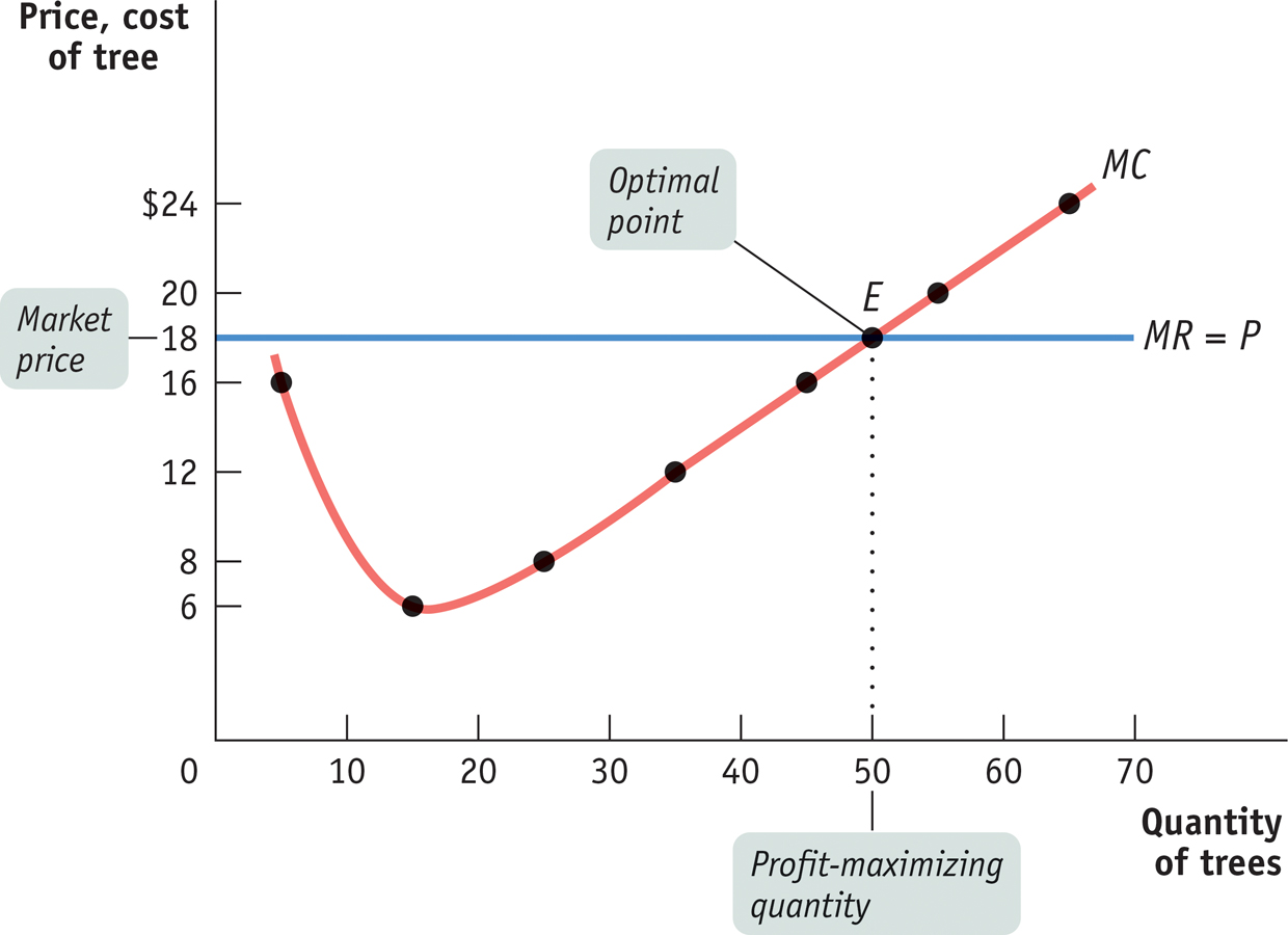
The Price-Taking Firm’s Profit-Maximizing Quantity of Output At the profit-maximizing quantity of output, the market price is equal to marginal cost. It is located at the point where the marginal cost curve crosses the marginal revenue curve, which is a horizontal line at the market price. Here, the profit-maximizing point is at an output of 50 trees, the output quantity at point E.
Note that whenever a firm is a price-taker, its marginal revenue curve is a horizontal line at the market price: it can sell as much as it likes at the market price. Regardless of whether it sells more or less, the market price is unaffected. In effect, the individual firm faces a horizontal, perfectly elastic demand curve for its output—an individual demand curve for its output that is equivalent to its marginal revenue curve. The marginal cost curve crosses the marginal revenue curve at point E where MC = MR. Sure enough, the quantity of output at E is 50 trees.
PITFALLS: WHAT IF MARGINAL REVENUE AND MARGINAL COST AREN’T EXACTLY EQUAL?
PITFALLS
WHAT IF MARGINAL REVENUE AND MARGINAL COST AREN’T EXACTLY EQUAL?
The optimal output rule says that to maximize profit, you should produce the quantity at which marginal revenue is equal to marginal cost. But what do you do if there is no output level at which marginal revenue equals marginal cost? In that case, you produce the largest quantity for which marginal revenue exceeds marginal cost. This is the case in Table 12-2 at an output of 50 trees. The simpler version of the optimal output rule applies when production involves large numbers, such as hundreds or thousands of units. In such cases marginal cost comes in small increments, and there is always a level of output at which marginal cost almost exactly equals marginal revenue.
Does this mean that the price-taking firm’s production decision can be entirely summed up as “produce up to the point where the marginal cost of production is equal to the price”? No, not quite. Before applying the profit-maximizing principle of marginal analysis to determine how much to produce, a potential producer must as a first step answer an “either-or” question: should it produce at all? If the answer to that question is yes, it then proceeds to the second step—a “how much” decision: maximizing profit by choosing the quantity of output at which marginal cost is equal to price.
To understand why the first step in the production decision involves an “either–or” question, we need to ask how we determine whether it is profitable or unprofitable to produce at all.
