Recall from Chapter 9 that a firm’s decision whether or not to stay in a given business depends on its economic profit—the measure of profit based on the opportunity cost of resources used in the business. To put it a slightly different way: in the calculation of economic profit, a firm’s total cost incorporates the implicit cost—the benefits forgone in the next best use of the firm’s resources—as well as the explicit cost in the form of actual cash outlays.

In contrast, accounting profit is profit calculated using only the explicit costs incurred by the firm. This means that economic profit incorporates the opportunity cost of resources owned by the firm and used in the production of output, while accounting profit does not.

A firm may make positive accounting profit while making zero or even negative economic profit. It’s important to understand clearly that a firm’s decision to produce or not, to stay in business or to close down permanently, should be based on economic profit, not accounting profit.

So we will assume, as we always do, that the cost numbers given in Tables 12-1 and 12-2 include all costs, implicit as well as explicit, and that the profit numbers in Table 12-1 are therefore economic profit. So what determines whether Noelle’s farm earns a profit or generates a loss? The answer is that, given the farm’s cost curves, whether or not it is profitable depends on the market price of trees—specifically, whether the market price is more or less than the farm’s minimum average total cost.

In Table 12-3 we calculate short-run average variable cost and short-run average total cost for Noelle’s farm. These are short-run values because we take fixed cost as given. (We’ll turn to the effects of changing fixed cost shortly.) The short-run average total cost curve, ATC, is shown in Figure 12-2, along with the marginal cost curve, MC, from Figure 12-1. As you can see, average total cost is minimized at point C, corresponding to an output of 40 trees—the minimum-cost output—and an average total cost of $14 per tree.

To see how these curves can be used to decide whether production is profitable or unprofitable, recall that profit is equal to total revenue minus total cost, TR − TC. This means:

We can also express this idea in terms of revenue and cost per unit of output. If we divide profit by the number of units of output, Q, we obtain the following expression for profit per unit of output:

TR/Q is average revenue, which is the market price. TC/Q is average total cost. So a firm is profitable if the market price for its product is more than the average total cost of the quantity the firm produces; a firm loses money if the market price is less than average total cost of the quantity the firm produces. This means:

Figure 12-3 illustrates this result, showing how the market price determines whether a firm is profitable. It also shows how profits are depicted graphically. Each panel shows the marginal cost curve, MC, and the short-run average total cost curve, ATC. Average total cost is minimized at point C. Panel (a) shows the case we have already analyzed, in which the market price of trees is $18 per tree. Panel (b) shows the case in which the market price of trees is lower, $10 per tree.

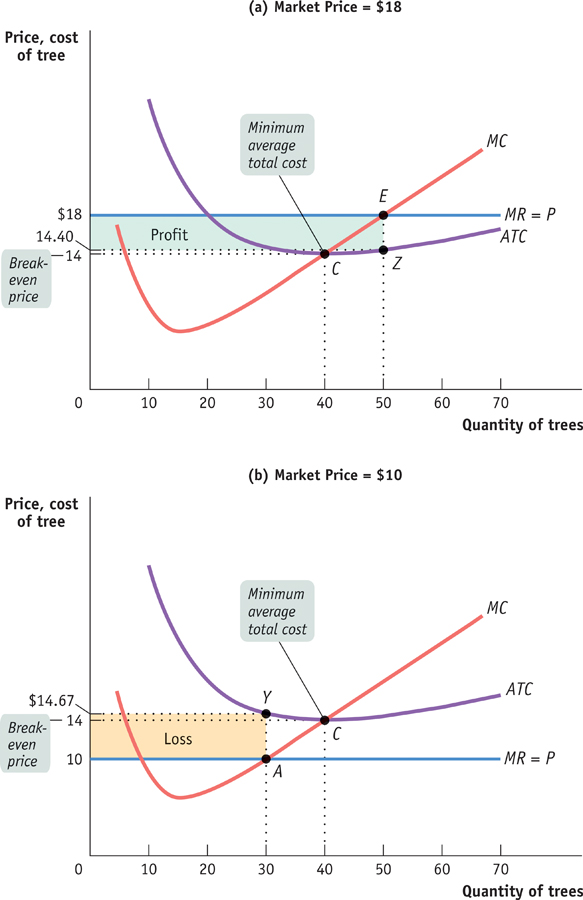
In panel (a), we see that at a price of $18 per tree the profit-maximizing quantity of output is 50 trees, indicated by point E, where the marginal cost curve, MC, intersects the marginal revenue curve—which for a price-taking firm is a horizontal line at the market price. At that quantity of output, average total cost is $14.40 per tree, indicated by point Z. Since the price per tree exceeds average total cost per tree, Noelle’s farm is profitable.

Noelle’s total profit when the market price is $18 is represented by the area of the shaded rectangle in panel (a). To see why, notice that total profit can be expressed in terms of profit per unit:

or, equivalently,

Profit = (P − ATC) × Q

since P is equal to TR/Q and ATC is equal to TC/Q. The height of the shaded rectangle in panel (a) corresponds to the vertical distance between points E and Z. It is equal to P − ATC = $18.00 − $14.40 = $3.60 per tree. The shaded rectangle has a width equal to the output: Q = 50 trees. So the area of that rectangle is equal to Noelle’s profit: 50 trees × $3.60 profit per tree = $180—the same number we calculated in Table 12-1.

What about the situation illustrated in panel (b)? Here the market price of trees is $10 per tree. Setting price equal to marginal cost leads to a profit-maximizing output of 30 trees, indicated by point A. At this output, Noelle has an average total cost of $14.67 per tree, indicated by point Y. At the profit-maximizing output quantity—30 trees—average total cost exceeds the market price. This means that Noelle’s farm generates a loss, not a profit.

How much does she lose by producing when the market price is $10? On each tree she loses ATC − P = $14.67 − $10.00 = $4.67, an amount corresponding to the vertical distance between points A and Y. And she would produce 30 trees, which corresponds to the width of the shaded rectangle. So the total value of the losses is $4.67 × 30 = $140.00 (adjusted for rounding error), an amount that corresponds to the area of the shaded rectangle in panel (b).

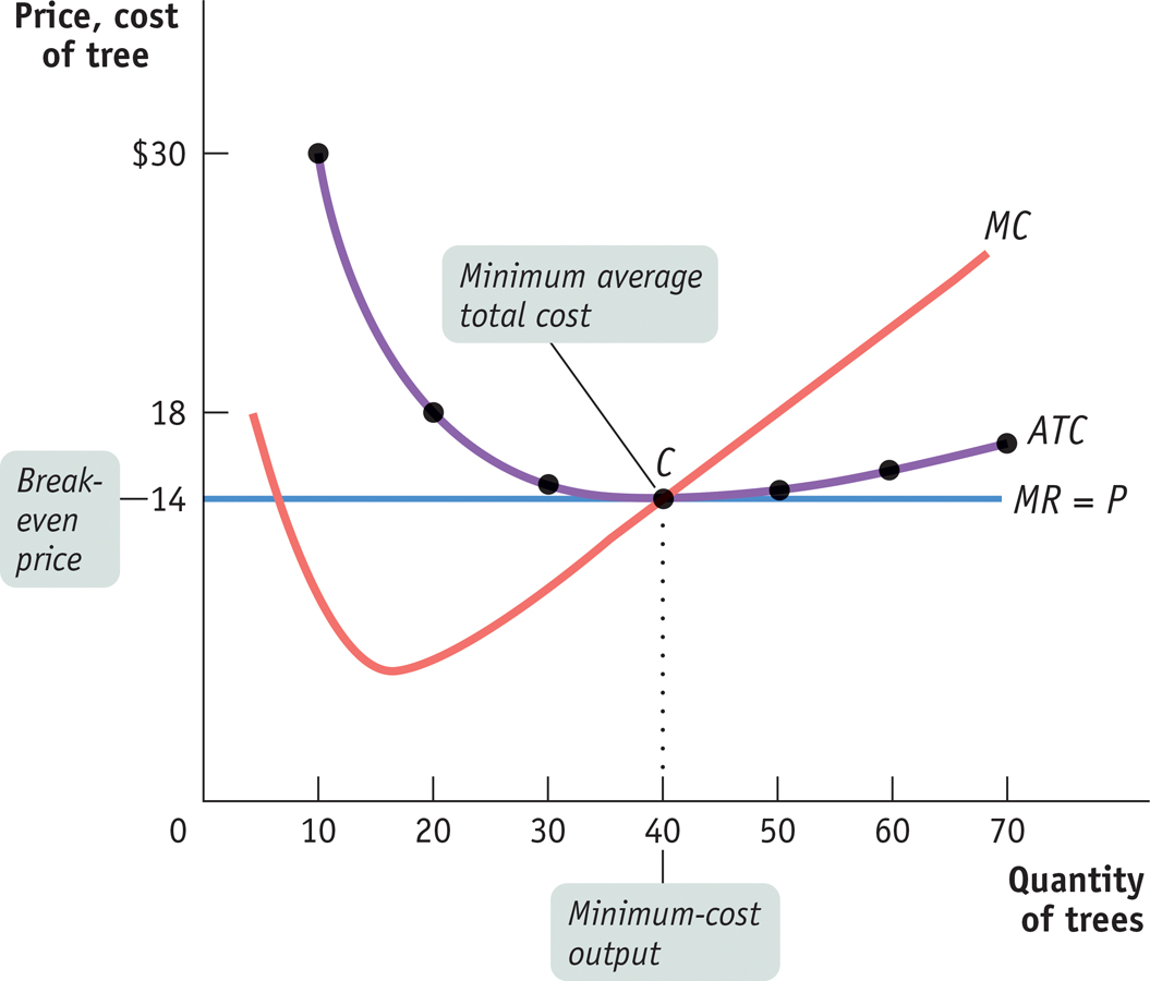
But how does a producer know, in general, whether or not its business will be profitable? It turns out that the crucial test lies in a comparison of the market price to the producer’s minimum average total cost. On Noelle’s farm, minimum average total cost, which is equal to $14, occurs at an output quantity of 40 trees, indicated by point C.

Whenever the market price exceeds minimum average total cost, the producer can find some output level for which the average total cost is less than the market price. In other words, the producer can find a level of output at which the firm makes a profit. So Noelle’s farm will be profitable whenever the market price exceeds $14. And she will achieve the highest possible profit by producing the quantity at which marginal cost equals the market price.

Conversely, if the market price is less than minimum average total cost, there is no output level at which price exceeds average total cost. As a result, the firm will be unprofitable at any quantity of output. As we saw, at a price of $10—an amount less than minimum average total cost—Noelle did indeed lose money. By producing the quantity at which marginal cost equals the market price, Noelle did the best she could, but the best that she could do was a loss of $140. Any other quantity would have increased the size of her loss.

The minimum average total cost of a price-taking firm is called its break-even price, the price at which it earns zero profit. (Recall that’s economic profit.) A firm will earn positive profit when the market price is above the break-even price, and it will suffer losses when the market price is below the break-even price. Noelle’s break-even price of $14 is the price at point C in Figures 12-2 and 12-3.

So the rule for determining whether a producer of a good is profitable depends on a comparison of the market price of the good to the producer’s breakeven price—its minimum average total cost: