Monopolistic Competition in the Short Run
We introduced the distinction between short-run and long-run equilibrium back in Chapter 12. The short-run equilibrium of an industry takes the number of firms as given. The long-run equilibrium, by contrast, is reached only after enough time has elapsed for firms to enter or exit the industry. To analyze monopolistic competition, we focus first on the short run and then on how an industry moves from the short run to the long run.
Panels (a) and (b) of Figure 15-1 show two possible situations that a typical firm in a monopolistically competitive industry might face in the short run. In each case, the firm looks like any monopolist: it faces a downward-sloping demand curve, which implies a downward-sloping marginal revenue curve.
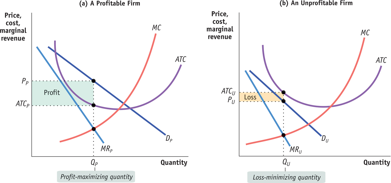
The Monopolistically Competitive Firm in the Short Run The firm in panel (a) can be profitable for some output quantities: the quantities for which its average total cost curve, ATC, lies below its demand curve, DP. The profit-maximizing output quantity is QP, the output at which marginal revenue, MRP, is equal to marginal cost, MC. The firm charges price PP and earns a profit, represented by the area of the green-shaded rectangle. The firm in panel (b), however, can never be profitable because its average total cost curve lies above its demand curve, DU, for every output quantity. The best that it can do if it produces at all is to produce quantity QU and charge price PU. This generates a loss, indicated by the area of the yellow-shaded rectangle. Any other output quantity results in a greater loss.
We assume that every firm has an upward-sloping marginal cost curve but that it also faces some fixed costs, so that its average total cost curve is U-shaped. This assumption doesn’t matter in the short run, but, as we’ll see shortly, it is crucial to understanding the long-run equilibrium.
In each case the firm, in order to maximize profit, sets marginal revenue equal to marginal cost. So how do these two figures differ? In panel (a) the firm is profitable; in panel (b) it is unprofitable. (Recall that we are referring always to economic profit, not accounting profit—that is, a profit given that all factors of production are earning their opportunity costs.)
In panel (a) the firm faces the demand curve DP and the marginal revenue curve MRP. It produces the profit-maximizing output QP, the quantity at which marginal revenue is equal to marginal cost, and sells it at the price PP. This price is above the average total cost at this output, ATCP. The firm’s profit is indicated by the area of the shaded rectangle.
In panel (b) the firm faces the demand curve DU and the marginal revenue curve MRU. It chooses the quantity QU at which marginal revenue is equal to marginal cost. However, in this case the price PU is below the average total cost ATCU; so at this quantity the firm loses money. Its loss is equal to the area of the shaded rectangle. Since QU is the profit-maximizing quantity—which means, in this case, the loss-minimizing quantity—there is no way for a firm in this situation to make a profit. We can confirm this by noting that at any quantity of output, the average total cost curve in panel (b) lies above the demand curve DU. Because ATC > P at all quantities of output, this firm always suffers a loss.
As this comparison suggests, the key to whether a firm with market power is profitable or unprofitable in the short run lies in the relationship between its demand curve and its average total cost curve. In panel (a) the demand curve DP crosses the average total cost curve, meaning that some of the demand curve lies above the average total cost curve. So there are some price-quantity combinations available at which price is higher than average total cost, indicating that the firm can choose a quantity at which it makes positive profit.
In panel (b), by contrast, the demand curve DU does not cross the average total cost curve—it always lies below it. So the price corresponding to each quantity demanded is always less than the average total cost of producing that quantity. There is no quantity at which the firm can avoid losing money.
These figures, showing firms facing downward-sloping demand curves and their associated marginal revenue curves, look just like ordinary monopoly analysis. The “competition” aspect of monopolistic competition comes into play, however, when we move from the short run to the long run.