Comparing Environmental Policies with an Example
Figure 16-3 shows a hypothetical industry consisting of only two plants, plant A and plant B. We’ll assume that plant A uses newer technology, giving it a lower cost of pollution reduction, while plant B uses older technology and has a higher cost of pollution reduction. Reflecting this difference, plant A’s marginal benefit of pollution curve, MBA, lies below plant B’s marginal benefit of pollution curve, MBB. Because it is more costly for plant B to reduce its pollution at any output quantity, an additional unit of pollution is worth more to plant B than to plant A.
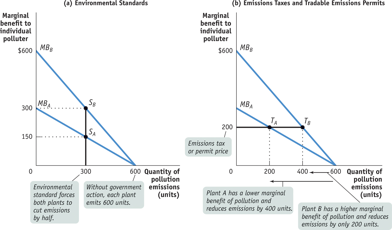
In the absence of government action, we know that polluters will pollute until the marginal social benefit of a unit of pollution is equal to zero. As a result, without government intervention each plant will pollute until its own marginal benefit of pollution is equal to zero. This corresponds to an emissions quantity of 600 units for each plant—
Now suppose that regulators decide that the overall pollution from this industry should be cut in half, from 1,200 units to 600 units. Panel (a) of Figure 16-3 shows this might be achieved with an environmental standard that requires each plant to cut its emissions in half, from 600 to 300 units. The standard has the desired effect of reducing overall emissions from 1,200 to 600 units but accomplishes it inefficiently.
As you can see from panel (a), the environmental standard leads plant A to produce at point SA, where its marginal benefit of pollution is $150, but plant B produces at point SB, where its marginal benefit of pollution is twice as high, $300.
This difference in marginal benefits between the two plants tells us that the same quantity of pollution can be achieved at lower total cost by allowing plant B to pollute more than 300 units but inducing plant A to pollute less. In fact, the efficient way to reduce pollution is to ensure that at the industry-
We can see from panel (b) how an emissions tax achieves exactly that result. Suppose both plant A and plant B pay an emissions tax of $200 per unit, so that the marginal cost of an additional unit of emissions to each plant is now $200 rather than zero. As a result, plant A produces at TA and plant B produces at TB. So plant A reduces its pollution more than it would under an inflexible environmental standard, cutting its emissions from 600 to 200 units; meanwhile, plant B reduces its pollution less, going from 600 to 400 units.
In the end, total pollution—
Panel (b) also illustrates why a system of tradable emissions permits also achieves an efficient allocation of pollution among the two plants. Assume that in the market for permits, the market price of a permit is $200 and each plant has 300 permits to start the system. Plant B, with the higher cost of pollution reduction, will buy 200 permits from Plant A, enough to allow it to emit 400 units. Correspondingly, Plant A, with the lower cost, will sell 200 of its permits to Plant B and emit only 200 units. Provided that the market price of a permit is the same as the optimal emissions tax, the two systems arrive at the same outcome.
!worldview! ECONOMICS in Action: Cap and Trade
Cap and Trade

The tradable emissions permit systems for both acid rain in the United States and greenhouse gases in the European Union are examples of cap and trade systems: the government sets a cap (a maximum amount of pollutant that can be emitted), issues tradable emissions permits, and enforces a yearly rule that a polluter must hold a number of permits equal to the amount of pollutant emitted. The goal is to set the cap low enough to generate environmental benefits, while giving polluters flexibility in meeting environmental standards and motivating them to adopt new technologies that will lower the cost of reducing pollution.
In 1994 the United States began a cap and trade system for the sulfur dioxide emissions that cause acid rain by issuing permits to power plants based on their historical consumption of coal. Thanks to the system, air pollutants in the United States decreased by more than 40% from 1990 to 2008, and by 2012 acid rain levels dropped to approximately 70% of their 1980 levels. Economists who have analyzed the sulfur dioxide cap and trade system point to another reason for its success: it would have been a lot more expensive—
The EU cap and trade scheme, begun in 2005 and covering all 28 member nations of the European Union, is the world’s only mandatory trading system for greenhouse gases. Other countries, like Australia and New Zealand, have adopted less comprehensive schemes.
According to the World Bank, the worldwide market for greenhouse gases—
Yet cap and trade systems are not silver bullets for the world’s pollution problems. Although they are appropriate for pollution that’s geographically dispersed, like sulfur dioxide and greenhouse gases, they don’t work for pollution that’s localized, like groundwater contamination. And there must be vigilant monitoring of compliance for the system to work. Finally, the amount of total reduction in pollution depends on the level of the cap, a critical issue illustrated by the troubles of the EU cap and trade scheme.
EU regulators, under industry pressure, allowed too many permits to be handed out when the system was created. By the spring of 2013 the price of a permit for a ton of greenhouse gas had fallen to 2.75 euros (about $3.70), less than a tenth of what experts believe is necessary to induce companies to switch to cleaner fuels like natural gas. The price of a permit was too low to alter polluters’ incentives and, not surprisingly, coal use in Europe boomed in 2012. Alarmed European Union legislators voted in the summer of 2013 to reduce the number of permits issued in future years in the hope of increasing the current price of a permit. There is evidence the reduction in permits has already altered polluters’ incentives. As of mid-
Quick Review
Governments often limit pollution with environmental standards. Generally, such standards are an inefficient way to reduce pollution because they are inflexible.
Environmental goals can be achieved efficiently in two ways: emissions taxes and tradable emissions permits. These methods are efficient because they are flexible, allocating more pollution reduction to those who can do it more cheaply. They also motivate polluters to adopt new pollution-
reducing technology. An emissions tax is a form of Pigouvian tax. The optimal Pigouvian tax is equal to the marginal social cost of pollution at the socially optimal quantity of pollution.
16-2
Question 16.3
Some opponents of tradable emissions permits object to them on the grounds that polluters that sell their permits benefit monetarily from their contribution to polluting the environment. Assess this argument.
Question 16.4
Explain the following.
Why an emissions tax smaller than or greater than the marginal social cost at QOPT leads to a smaller total surplus compared to the total surplus generated if the emissions tax had been set optimally
Why a system of tradable emissions permits that sets the total quantity of allowable pollution higher or lower than QOPT leads to a smaller total surplus compared to the total surplus generated if the number of permits had been set optimally.
Solutions appear at back of book.