If we maintain the assumption that the markets for goods and services are perfectly competitive, the result that we derived for the labor market also applies to other factors of production. Suppose, for example, that a farmer is considering whether to rent an additional acre of land for the next year. He or she will compare the cost of renting that acre with the value of the additional output generated by employing an additional acre—the value of the marginal product of an acre of land. To maximize profit, the farmer must employ land up to the point at which the value of the marginal product of an acre of land is equal to the rental rate per acre.

What if the farmer already owns the land? We already saw the answer in Chapter 9, which dealt with economic decisions: even if you own land, there is an implicit cost—the opportunity cost—of using it for a given activity, because it could be used for something else, such as renting it out to other farmers at the market rental rate. So a profit-maximizing producer employs additional acres of land up to the point at which the cost of the last acre employed, explicit or implicit, is equal to the value of the marginal product of that acre.

The same is true for capital. The explicit or implicit cost of using a unit of land or capital for a set period of time is called its rental rate. In general, a unit of land or capital is employed up to the point at which that unit’s value of the marginal product is equal to its rental rate over that time period. How are the rental rates for land and capital determined? By the equilibria in the land market and the capital market, of course. Figure 19-7 illustrates those outcomes.

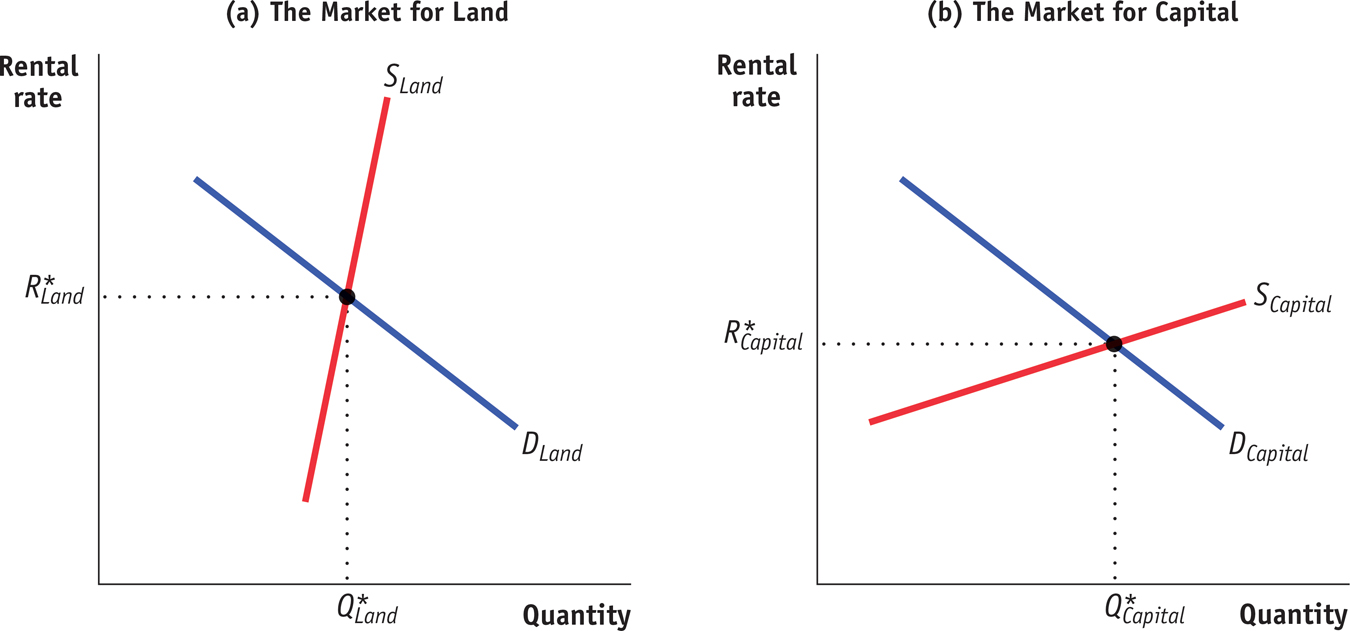
Panel (a) shows the equilibrium in the market for land. Summing over the individual demand curves for land of all producers gives us the market demand curve for land. Due to diminishing returns, the demand curve slopes downward, like the demand curve for labor. As we have drawn it, the supply curve of land is relatively steep and therefore relatively inelastic. This reflects the fact that finding new supplies of land for production is typically difficult and expensive—for example, creating new farmland through expensive irrigation. The equilibrium rental rate for land, , and the equilibrium quantity of land employed in production, , are given by the intersection of the two curves.

Panel (b) shows the equilibrium in the market for capital. In contrast to the supply curve for land, the supply curve for capital is relatively elastic. That’s because the supply of capital is relatively responsive to price: capital is paid for with funds that come from the savings of investors, and the amount of savings that investors make available is relatively responsive to the rental rate for capital. The equilibrium rental rate for capital, , and the equilibrium quantity of capital employed in production, , are given by the intersection of the two curves.