To understand how diminishing marginal utility gives rise to risk aversion, we need to look not only at the Lees’ medical costs but also at how those costs affect the income the family has left after medical expenses. Let’s assume the family knows that it will have an income of $30,000 next year. If the family has no medical expenses, it will be left with all of that income. If its medical expenses are $10,000, its income after medical expenses will be only $20,000. Since we have assumed that there is an equal chance of these two outcomes, the expected value of the Lees’ income after medical expenses is (0.5 × $30,000) + (0.5 × $20,000) = $25,000. At times we will simply refer to this as expected income.

But as we’ll now see, if the family’s utility function has the shape typical of most families’, its expected utility—the expected value of its total utility given uncertainty about future outcomes—is less than it would be if the family didn’t face any risk and knew with certainty that its income after medical expenses would be $25,000.

To see why, we need to look at how total utility depends on income. Panel (a) of Figure 20-1 shows a hypothetical utility function for the Lee family, where total utility depends on income—the amount of money the Lees have available for consumption of goods and services (after they have paid any medical bills). The table within the figure shows how the family’s total utility varies over the income range of $20,000 to $30,000. As usual, the utility function slopes upward, because more income leads to higher total utility. Notice as well that the curve gets flatter as we move up and to the right, which reflects diminishing marginal utility.

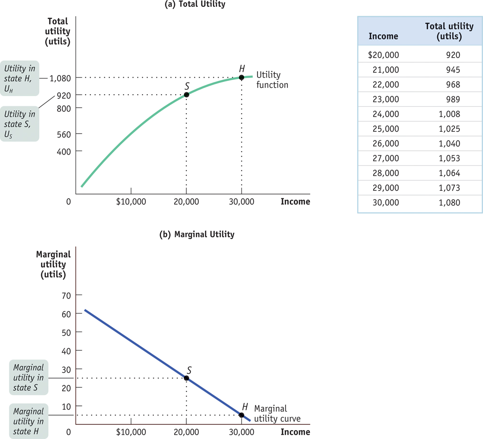
In Chapter 10 we applied the principle of diminishing marginal utility to individual goods and services: each successive unit of a good or service that a consumer purchases adds less to his or her total utility. The same principle applies to income used for consumption: each successive dollar of income adds less to total utility than the previous dollar. Panel (b) shows how marginal utility varies with income, confirming that marginal utility of income falls as income rises. As we’ll see in a moment, diminishing marginal utility is the key to understanding the desire of individuals to reduce risk.

To analyze how a person’s utility is affected by risk, economists start from the assumption that individuals facing uncertainty maximize their expected utility. We can use the data in Figure 20-1 to calculate the Lee family’s expected utility. We’ll first do the calculation assuming that the Lees have no insurance, and then we’ll recalculate it assuming that they have purchased insurance.

Without insurance, if the Lees are lucky and don’t incur any medical expenses, they will have an income of $30,000, generating total utility of 1,080 utils. But if they have no insurance and are unlucky, incurring $10,000 in medical expenses, they will have just $20,000 of their income to spend on consumption and total utility of only 920 utils. So without insurance, the family’s expected utility is (0.5 × 1,080) + (0.5 × 920) = 1,000 utils.

Now let’s suppose that an insurance company offers to pay whatever medical expenses the family incurs during the next year in return for a premium—a payment to the insurance company—of $5,000. Note that the amount of the premium in this case is equal to the expected value of the Lees’ medical expenses—the expected value of their future claim against the policy. An insurance policy with this feature, for which the premium is equal to the expected value of the claim, has a special name—a fair insurance policy.

If the family purchases this fair insurance policy, the expected value of its income available for consumption is the same as it would be without insurance: $25,000—that is, $30,000 minus the $5,000 premium. But the family’s risk has been eliminated: the family has an income available for consumption of $25,000 for sure, which means that it receives the utility level associated with an income of $25,000.

Reading from the table in Figure 20-1, we see that this utility level is 1,025 utils. Or to put it a slightly different way, their expected utility with insurance is 1 × 1,025 = 1,025 utils, because with insurance they will receive a utility of 1,025 utils with a probability of 1. And this is higher than the level of expected utility without insurance—only 1,000 utils. So by eliminating risk through the purchase of a fair insurance policy, the family increases its expected utility even though its expected income hasn’t changed.

The calculations for this example are summarized in Table 20-1. This example shows that the Lees, like most people in real life, are risk-averse: they will choose to reduce the risk they face when the cost of that reduction leaves the expected value of their income or wealth unchanged. So the Lees, like most people, will be willing to buy fair insurance.

You might think that this result depends on the specific numbers we have chosen. In fact, however, the proposition that purchase of a fair insurance policy increases expected utility depends on only one assumption: diminishing marginal utility. The reason is that with diminishing marginal utility, a dollar gained when income is low adds more to utility than a dollar gained when income is high.

That is, having an additional dollar matters more when you are facing hard times than when you are facing good times. And as we will shortly see, a fair insurance policy is desirable because it transfers a dollar from high-income states (where it is valued less) to low-income states (where it is valued more).

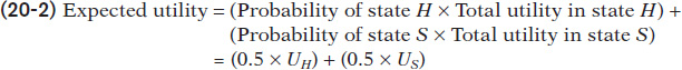
But first, let’s see how diminishing marginal utility leads to risk aversion by examining expected utility more closely. In the case of the Lee family, there are two states of the world; let’s call them H and S, for healthy and sick. In state H the family has no medical expenses; in state S it has $10,000 in medical expenses. Let’s use the symbols U_H and U_S to represent the Lee family’s total utility in each state. Then the family’s expected utility is:

The fair insurance policy reduces the family’s income available for consumption in state H by $5,000, but it increases it in state S by the same amount. As we’ve just seen, we can use the utility function to directly calculate the effects of these changes on expected utility. But as we have also seen in many other contexts, we gain more insight into individual choice by focusing on marginal utility.

To use marginal utility to analyze the effects of fair insurance, let’s imagine introducing the insurance a bit at a time, say in 5,000 small steps. At each of these steps, we reduce income in state H by $1 and simultaneously increase income in state S by $1. At each of these steps, total utility in state H falls by the marginal utility of income in that state but total utility in state S rises by the marginal utility of income in that state.

Now look again at panel (b) of Figure 20-1, which shows how marginal utility varies with income. Point S shows marginal utility when the Lee family’s income is $20,000; point H shows marginal utility when income is $30,000. Clearly, marginal utility is higher when income after medical expenses is low. Because of diminishing marginal utility, an additional dollar of income adds more to total utility when the family has low income (point S) than when it has high income (point H).

This tells us that the gain in expected utility from increasing income in state S is larger than the loss in expected utility from reducing income in state H by the same amount. So at each step of the process of reducing risk, by transferring $1 of income from state H to state S, expected utility increases. This is the same as saying that the family is risk-averse; that is, risk aversion is a result of diminishing marginal utility.

Almost everyone is risk-averse, because almost everyone has diminishing marginal utility. But the degree of risk aversion varies among individuals—some people are more risk-averse than others. To illustrate this point, Figure 20-2 compares two individuals, Danny and Mel. We suppose that each of them earns the same income now but is confronted with the possibility of earning either $1,000 more or $1,000 less.

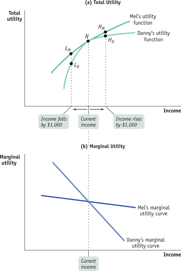
Panel (a) of Figure 20-2 shows how each individual’s total utility would be affected by the change in income. Danny would gain very few utils from a rise in income, which moves him from N to H_D, but lose a large number of utils from a fall in income, which moves him from N to L_D. That is, he is highly risk-averse. This is reflected in panel (b) by his steeply declining marginal utility curve.

Mel, though, as shown in panel (a), would gain almost as many utils from higher income, which moves him from N to H_M, as he would lose from lower income, which moves him from N to L_M. He is barely risk-averse at all. This is reflected in his marginal utility curve in panel (b), which is almost horizontal. So, other things equal, Danny will gain a lot more utility from insurance than Mel will. Someone who is completely insensitive to risk is called risk-neutral.

Individuals differ in risk aversion for two main reasons: differences in preferences and differences in initial income or wealth.

Differences in risk aversion have an important consequence: they affect how much an individual is willing to pay to avoid risk.