Measuring the Price Elasticity of Supply
The price elasticity of supply is a measure of the responsiveness of the quantity of a good supplied to the price of that good. It is the ratio of the percent change in the quantity supplied to the percent change in the price as we move along the supply curve.
The price elasticity of supply is defined the same way as the price elasticity of demand (although there is no minus sign to be eliminated here):

The only difference is that now we consider movements along the supply curve rather than movements along the demand curve.
Suppose that the price of tomatoes rises by 10%. If the quantity of tomatoes supplied also increases by 10% in response, the price elasticity of supply of tomatoes is 1 (10%/10%) and supply is unit-
As in the case of demand, the extreme values of the price elasticity of supply have a simple graphical representation. Panel (a) of Figure 6-6 shows the supply of cell phone frequencies, the portion of the radio spectrum that is suitable for sending and receiving cell phone signals. Governments own the right to sell the use of this part of the radio spectrum to cell phone operators inside their borders. But governments can’t increase or decrease the number of cell phone frequencies that they have to offer—
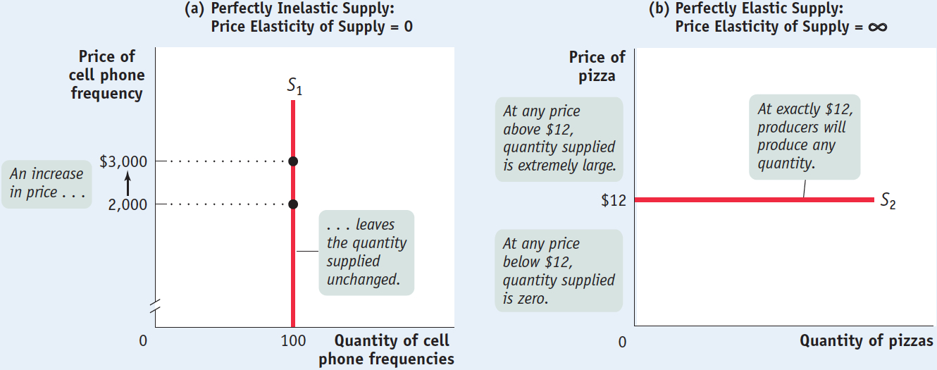
There is perfectly inelastic supply when the price elasticity of supply is zero, so that changes in the price of the good have no effect on the quantity supplied. A perfectly inelastic supply curve is a vertical line.
So the supply curve for cell phone frequencies is a vertical line, which we have assumed is set at the quantity of 100 frequencies. As you move up and down that curve, the change in the quantity supplied by the government is zero, whatever the change in price. So panel (a) illustrates a case in which the price elasticity of supply is zero. This is a case of perfectly inelastic supply.
Panel (b) shows the supply curve for pizza. We suppose that it costs $12 to produce a pizza, including all opportunity costs. At any price below $12, it would be unprofitable to produce pizza and all the pizza parlors in America would go out of business. Alternatively, there are many producers who could operate pizza parlors if they were profitable. The ingredients—
There is perfectly elastic supply when even a tiny increase or reduction in the price will lead to very large changes in the quantity supplied, so that the price elasticity of supply is infinite. A perfectly elastic supply curve is a horizontal line.
Since even a tiny increase in the price would lead to a huge increase in the quantity supplied, the price elasticity of supply would be more or less infinite. This is a case of perfectly elastic supply.
As our cell phone frequencies and pizza examples suggest, real-