How Elastic Is Elastic?
As a first step toward classifying price elasticities of demand, let’s look at the extreme cases.
First, consider the demand for a good when people pay no attention to the price—
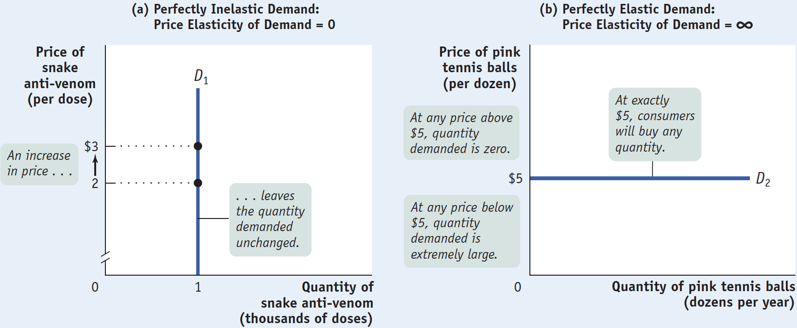
Demand is perfectly inelastic when the quantity demanded does not respond at all to changes in the price. When demand is perfectly inelastic, the demand curve is a vertical line.
The opposite extreme occurs when even a tiny rise in the price will cause the quantity demanded to drop to zero or even a tiny fall in the price will cause the quantity demanded to get extremely large.
Demand is perfectly elastic when any price increase will cause the quantity demanded to drop to zero. When demand is perfectly elastic, the demand curve is a horizontal line.
Panel (b) of Figure 6-2 shows the case of pink tennis balls; we suppose that tennis players really don’t care what color their balls are and that other colors, such as neon green and vivid yellow, are available at $5 per dozen balls. In this case, consumers will buy no pink balls if they cost more than $5 per dozen but will buy only pink balls if they cost less than $5. The demand curve will therefore be a horizontal line at a price of $5 per dozen balls. As you move back and forth along this line, there is a change in the quantity demanded but no change in the price. Roughly speaking, when you divide a number by zero, you get infinity, denoted by the symbol ∞. So a horizontal demand curve implies an infinite price elasticity of demand. When the price elasticity of demand is infinite, economists say that demand is perfectly elastic.
Demand is elastic if the price elasticity of demand is greater than 1, inelastic if the price elasticity of demand is less than 1, and unit-
The price elasticity of demand for the vast majority of goods is somewhere between these two extreme cases. Economists use one main criterion for classifying these intermediate cases: they ask whether the price elasticity of demand is greater or less than 1. When the price elasticity of demand is greater than 1, economists say that demand is elastic. When the price elasticity of demand is less than 1, they say that demand is inelastic. The borderline case is unit-
To see why a price elasticity of demand equal to 1 is a useful dividing line, let’s consider a hypothetical example: a toll bridge operated by the state highway department. Other things equal, the number of drivers who use the bridge depends on the toll, the price the highway department charges for crossing the bridge: the higher the toll, the fewer the drivers who use the bridge.
Figure 6-3 shows three hypothetical demand curves—
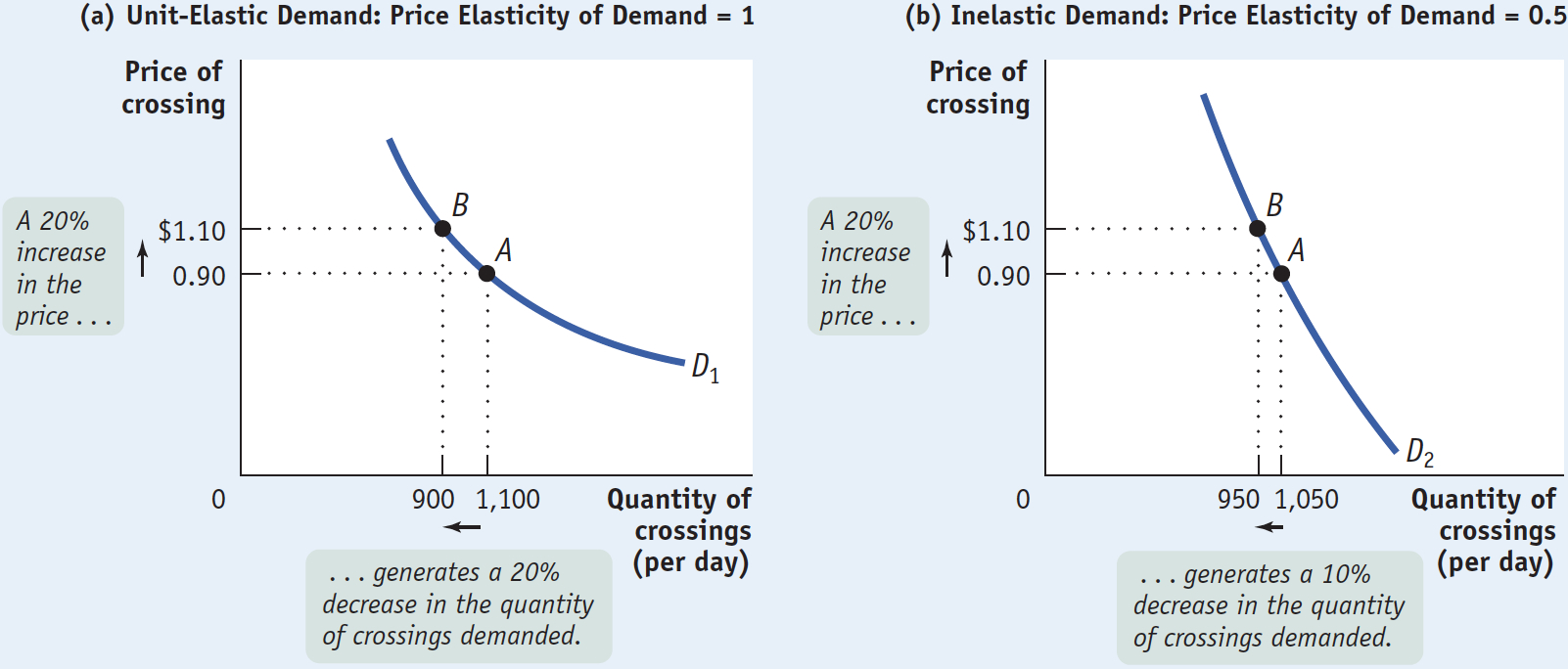
Panel (a) shows what happens when the toll is raised from $0.90 to $1.10 and the demand curve is unit-
Panel (b) shows a case of inelastic demand when the toll is raised from $0.90 to $1.10. The same 20% price rise reduces the quantity demanded from 1,050 to 950. That’s only a 10% decline, so in this case the price elasticity of demand is 10%/20% = 0.5.
Panel (c) shows a case of elastic demand when the toll is raised from $0.90 to $1.10. The 20% price increase causes the quantity demanded to fall from 1,200 to 800—
The total revenue is the total value of sales of a good or service. It is equal to the price multiplied by the quantity sold.
Why does it matter whether demand is unit-

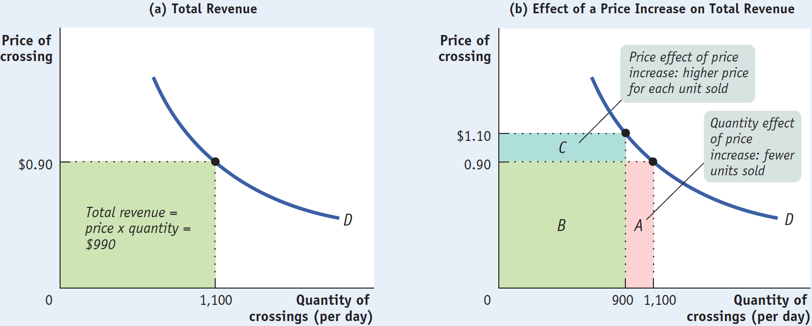
Total revenue has a useful graphical representation that can help us understand why knowing the price elasticity of demand is crucial when we ask whether a price rise will increase or reduce total revenue. Panel (a) of Figure 6-4 shows the same demand curve as panel (a) of Figure 6-3. We see that 1,100 drivers will use the bridge if the toll is $0.90. So the total revenue at a price of $0.90 is $0.90 × 1,100 = $990. This value is equal to the area of the green rectangle, which is drawn with the bottom left corner at the point (0, 0) and the top right corner at (1,100, 0.90). In general, the total revenue at any given price is equal to the area of a rectangle whose height is the price and whose width is the quantity demanded at that price.
To get an idea of why total revenue is important, consider the following scenario. Suppose that the toll on the bridge is currently $0.90 but that the highway department must raise extra money for road repairs. One way to do this is to raise the toll on the bridge. But this plan might backfire, since a higher toll will reduce the number of drivers who use the bridge. And if traffic on the bridge dropped a lot, a higher toll would actually reduce total revenue instead of increasing it. So it’s important for the highway department to know how drivers will respond to a toll increase.
We can see graphically how the toll increase affects total bridge revenue by examining panel (b) of Figure 6-4. At a toll of $0.90, total revenue is given by the sum of the areas A and B. After the toll is raised to $1.10, total revenue is given by the sum of areas B and C. So when the toll is raised, revenue represented by area A is lost but revenue represented by area C is gained.
These two areas have important interpretations. Area C represents the revenue gain that comes from the additional $0.20 paid by drivers who continue to use the bridge. That is, the 900 who continue to use the bridge contribute an additional $0.20 × 900 = $180 per day to total revenue, represented by area C. But 200 drivers who would have used the bridge at a price of $0.90 no longer do so, generating a loss to total revenue of $0.90 × 200 = $180 per day, represented by area A. (In this particular example, because demand is unit-

Except in the rare case of a good with perfectly elastic or perfectly inelastic demand, when a seller raises the price of a good, two countervailing effects are present:
A price effect: After a price increase, each unit sold sells at a higher price, which tends to raise revenue.
A quantity effect: After a price increase, fewer units are sold, which tends to lower revenue.
But then, you may ask, what is the ultimate net effect on total revenue: does it go up or down? The answer is that, in general, the effect on total revenue can go either way—
The price elasticity of demand tells us what happens to total revenue when price changes: its size determines which effect—
If demand for a good is unit-
elastic (the price elasticity of demand is 1), an increase in price does not change total revenue. In this case, the quantity effect and the price effect exactly offset each other. If demand for a good is inelastic (the price elasticity of demand is less than 1), a higher price increases total revenue. In this case, the quantity effect is weaker than the price effect.
If demand for a good is elastic (the price elasticity of demand is greater than 1), an increase in price reduces total revenue. In this case, the quantity effect is stronger than the price effect.
Table 6-2 shows how the effect of a price increase on total revenue depends on the price elasticity of demand, using the same data as in Figure 6-3. An increase in the price from $0.90 to $1.10 leaves total revenue unchanged at $990 when demand is unit-
|
Price of toll = $0.90 |
Price of toll = $1.10 |
|
|---|---|---|
|
Unit- (price elasticity of demand = 1) |
||
|
Quantity demanded |
1,100 |
900 |
|
Total revenue |
$990 |
$990 |
|
Inelastic demand (price elasticity of demand = 0.5) |
||
|
Quantity demanded |
1,050 |
950 |
|
Total revenue |
$945 |
$1,045 |
|
Elastic demand (price elasticity of demand = 2) |
||
|
Quantity demanded |
1,200 |
800 |
|
Total revenue |
$1,080 |
$880 |
TABLE 6-
The price elasticity of demand also predicts the effect of a fall in price on total revenue. When the price falls, the same two countervailing effects are present, but they work in the opposite directions as compared to the case of a price rise. There is the price effect of a lower price per unit sold, which tends to lower revenue. This is countered by the quantity effect of more units sold, which tends to raise revenue. Which effect dominates depends on the price elasticity. Here is a quick summary:
When demand is unit-
elastic, the two effects exactly balance; so a fall in price has no effect on total revenue. When demand is inelastic, the quantity effect is dominated by the price effect; so a fall in price reduces total revenue.
When demand is elastic, the quantity effect dominates the price effect; so a fall in price increases total revenue.