Marginal Cost
We’ll assume that each additional year of schooling costs Alex $10,000 in explicit costs—
Unlike Alex’s explicit costs, which are constant (that is, the same each year), Alex’s implicit cost changes each year. That’s because each year he spends in school leaves him better trained than the year before; and the better trained he is, the higher the salary he can command. Consequently, the income he forgoes by not working rises each additional year he stays in school. In other words, the greater the number of years Alex has already spent in school, the higher his implicit cost of another year of school.
Table 9-4 contains the data on how Alex’s cost of an additional year of schooling changes as he completes more years. The second column shows how his total cost of schooling changes as the number of years he has completed increases. For example, Alex’s first year has a total cost of $30,000: $10,000 in explicit costs of tuition and the like as well as $20,000 in forgone salary.
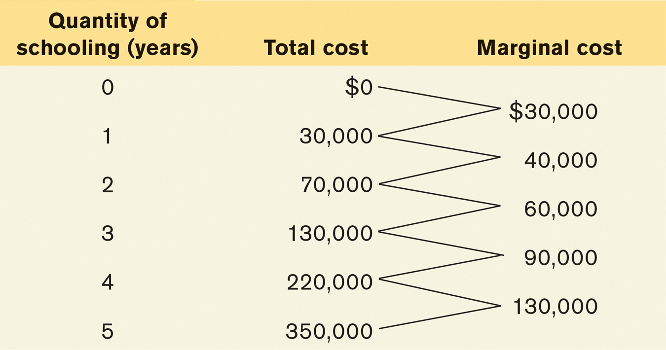
The second column also shows that the total cost of attending two years is $70,000: $30,000 for his first year plus $40,000 for his second year. During his second year in school, his explicit costs have stayed the same ($10,000) but his implicit cost of forgone salary has gone up to $30,000. That’s because he’s a more valuable worker with one year of schooling under his belt than with no schooling.
Likewise, the total cost of three years of schooling is $130,000: $30,000 in explicit cost for three years of tuition plus $100,000 in implicit cost of three years of forgone salary. The total cost of attending four years is $220,000, and $350,000 for five years.
The marginal cost of producing a good or service is the additional cost incurred by producing one more unit of that good or service.
The change in Alex’s total cost of schooling when he goes to school an additional year is his marginal cost of the one-
Production of a good or service has increasing marginal cost when each additional unit costs more to produce than the previous one.
As already mentioned, the third column of Table 9-4 shows Alex’s marginal costs of more years of schooling, which have a clear pattern: they are increasing. They go from $30,000, to $40,000, to $60,000, to $90,000, and finally to $130,000 for the fifth year of schooling. That’s because each year of schooling would make Alex a more valuable and highly paid employee if he were to work. As a result, for-
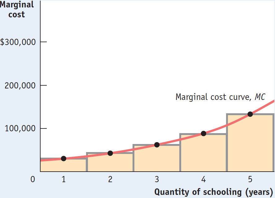
The marginal cost curve shows how the cost of producing one more unit depends on the quantity that has already been produced.
Figure 9-1 shows the marginal cost curve, a graphical representation of Alex’s marginal costs. The height of each shaded bar corresponds to the marginal cost of a given year of schooling. The red line connecting the dots at the midpoint of the top of each bar is Alex’s marginal cost curve. Alex has an upward-
Production of a good or service has constant marginal cost when each additional unit costs the same to produce as the previous one.
Although increasing marginal cost is a frequent phenomenon in real life, it’s not the only possibility. Constant marginal cost occurs when the cost of producing an additional unit is the same as the cost of producing the previous unit. Plant nurseries, for example, typically have constant marginal cost—
Production of a good or service has decreasing marginal cost when each additional unit costs less to produce than the previous one.
There can also be decreasing marginal cost, which occurs when marginal cost falls as the number of units produced increases. With decreasing marginal cost, the marginal cost line is downward sloping. Decreasing marginal cost is often due to learning effects in production: for complicated tasks, such as assembling a new model of a car, workers are often slow and mistake-
Finally, for the production of some goods and services the shape of the marginal cost curve changes as the number of units produced increases. For example, auto production is likely to have decreasing marginal costs for the first batch of cars produced as workers iron out kinks and mistakes in production. Then production has constant marginal costs for the next batch of cars as workers settle into a predictable pace.
But at some point, as workers produce more cars, marginal cost begins to increase as they run out of factory floor space and the auto company incurs costly overtime wages. This gives rise to what we call a “swoosh”-shaped marginal cost curve—
PITFALLS: TOTAL COST VERSUS MARGINAL COST
TOTAL COST VERSUS MARGINAL COST
It can be easy to conclude that marginal cost and total cost must always move in the same direction. That is, if total cost is rising, then marginal cost must also be rising. Or if marginal cost is falling, then total cost must be falling as well. But the following example shows that this conclusion is wrong.
Let’s consider the example of auto production, which, as we mentioned earlier, is likely to involve learning effects. Suppose that for the first batch of cars of a new model, each car costs $10,000 to assemble. As workers gain experience with the new model, they become better at production. As a result, the per-
In this example, marginal cost is decreasing over batches one through four, falling from $10,000 to $5,000. However, it’s important to note that total cost is still increasing over the entire production run because marginal cost is greater than zero.
To see this point, assume that each batch consists of 100 cars. Then the total cost of producing the first batch is 100 × $10,000 = $1,000,000. The total cost of producing the first and second batch of cars is $1,000,000 + (100 × $8,000) = $1,800,000. Likewise, the total cost of producing the first, second, and third batch is $1,800,000 + (100 × $6,500) = $2,450,000, and so on. As you can see, although marginal cost is decreasing over the first few batches of cars, total cost is increasing over the same batches.
This shows us that totals and marginals can sometimes move in opposite directions. So it is wrong to assert that they always move in the same direction. What we can assert is that total cost increases whenever marginal cost is positive, regardless of whether marginal cost is increasing or decreasing.