Marginal Analysis
Table 9-6 shows the marginal cost and marginal benefit numbers from Tables 9-4 and 9-5. It also adds an additional column: the additional profit to Alex from staying in school one more year, equal to the difference between the marginal benefit and the marginal cost of that additional year in school. (Remember that it is Alex’s economic profit that we care about, not his accounting profit.) We can now use Table 9-6 to determine how many additional years of schooling Alex should undertake in order to maximize his total profit.
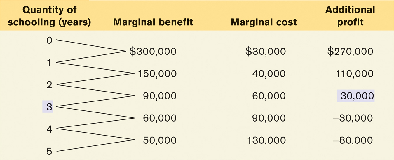
First, imagine that Alex chooses not to attend any additional years of school. We can see from column 4 that this is a mistake if Alex wants to achieve the highest total profit from his schooling—
Now, let’s consider whether Alex should attend the second year of school. The additional profit from the second year is $110,000, so Alex should attend the second year as well. What about the third year? The additional profit from that year is $30,000; so, yes, Alex should attend the third year as well.
What about a fourth year? In this case, the additional profit is negative: it is
−$30,000. Alex loses $30,000 of the value of his lifetime earnings if he attends the fourth year. Clearly, Alex is worse off by attending the fourth additional year rather than taking a job. And the same is true for the fifth year as well: it has a negative additional profit of −$80,000.
The optimal quantity is the quantity that generates the highest possible total profit.
What have we learned? That Alex should attend three additional years of school and stop at that point. Although the first, second, and third years of additional schooling increase the value of his lifetime earnings, the fourth and fifth years diminish it. So three years of additional schooling lead to the quantity that generates the maximum possible total profit. It is what economists call the optimal quantity—the quantity that generates the maximum possible total profit.
Figure 9-3 shows how the optimal quantity can be determined graphically. Alex’s marginal benefit and marginal cost curves are shown together. If Alex chooses fewer than three additional years (that is, years 0, 1, or 2), he will choose a level of schooling at which his marginal benefit curve lies above his marginal cost curve. He can make himself better off by staying in school.
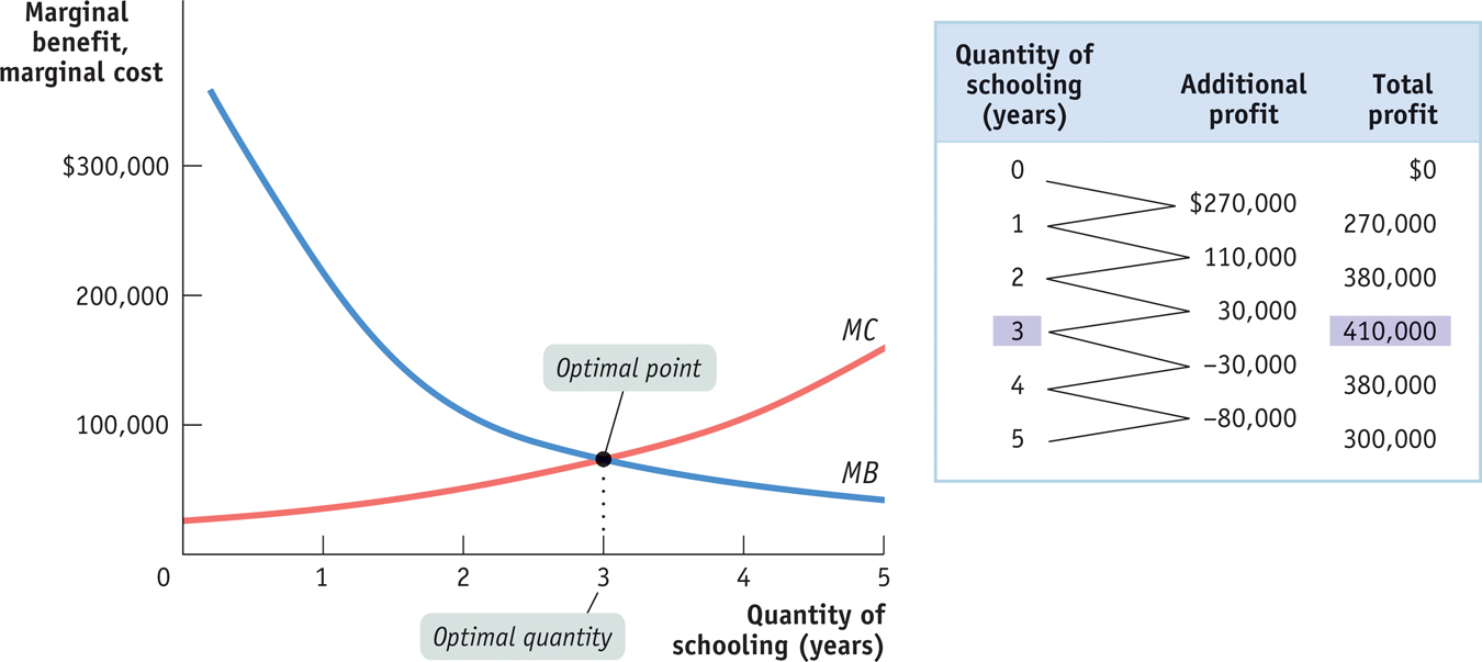
If instead he chooses more than three additional years (years 4 or 5), he will choose a level of schooling at which his marginal benefit curve lies below his marginal cost curve. He can make himself better off by choosing not to attend the additional year of school and taking a job instead.
The table in Figure 9-3 confirms our result. The second column repeats information from Table 9-6, showing Alex’s marginal benefit minus marginal cost—
For example, Alex’s profit from additional years of schooling is $270,000 for the first year and $110,000 for the second year. So the total profit for two additional years of schooling is $270,000 + $110,000 = $380,000. Similarly, the total profit for three additional years is $270,000 + $110,000 + $30,000 = $410,000. Our claim that three years is the optimal quantity for Alex is confirmed by the data in the table in Figure 9-3: at three years of additional schooling, Alex reaps the greatest total profit, $410,000.
Alex’s decision problem illustrates how you go about finding the optimal quantity when the choice involves a small number of quantities. (In this example, one through five years.) With small quantities, the rule for choosing the optimal quantity is: increase the quantity as long as the marginal benefit from one more unit is greater than the marginal cost, but stop before the marginal benefit becomes less than the marginal cost.
In contrast, when a “how much” decision involves relatively large quantities, the rule for choosing the optimal quantity simplifies to this: The optimal quantity is the quantity at which marginal benefit is equal to marginal cost.
To see why this is so, consider the example of a farmer who finds that her optimal quantity of wheat produced is 5,000 bushels. Typically, she will find that in going from 4,999 to 5,000 bushels, her marginal benefit is only very slightly greater than her marginal cost—
According to the profit-
So a simple rule for her in choosing the optimal quantity of wheat is to produce the quantity at which the difference between marginal benefit and marginal cost is approximately zero—
Now we are ready to state the general rule for choosing the optimal quantity—
Portion Sizes
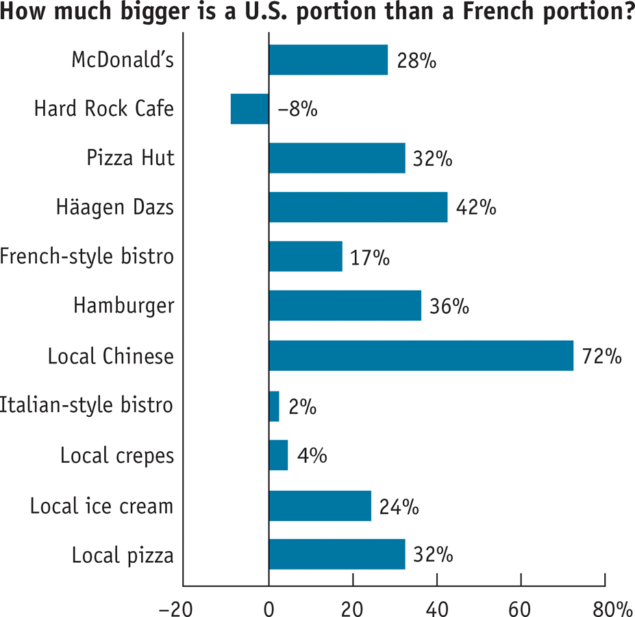
Health experts call it the “French Paradox.” If you think French food is fattening, you’re right: the French diet is, on average, higher in fat than the American diet. Yet the French themselves are considerably thinner than we are: in 2012, 15% of French adults were classified as obese, compared with 34.9% of Americans.
What’s the secret? It seems that the French simply eat less, largely because they eat smaller portions. This chart compares average portion sizes at food establishments in Paris and Philadelphia. In four cases, researchers looked at portions served by the same chain; in the other cases, they looked at comparable establishments, such as local pizza parlors. In every case but one, U.S. portions were bigger, often much bigger.
Why are American portions so big? Because food is cheaper in the United States. At the margin, it makes sense for restaurants to offer big portions, since the additional cost of the larger portion is relatively small. As a news article notes: “So while it may cost a restaurant a few pennies to offer 25% more French fries, it can raise its prices much more than a few cents.” Larger portions, then, lead to higher checks at U.S. restaurants. And if you have ever wondered why dieting seems to be a uniquely American obsession, the principle of marginal analysis can help provide the answer: it’s to counteract the effects of our larger portion sizes.
Source: Paul Rozin, Kimberly Kabnick, Erin Pete, Claude Fischler, and Christy Shields, “The Ecology of Eating,” Psychological Science 14 (September 2003): 450–
PITFALLS: MUDDLED AT THE MARGIN
MUDDLED AT THE MARGIN
The idea of setting marginal benefit equal to marginal cost sometimes confuses people. Aren’t we trying to maximize the difference between benefits and costs? Yes. And don’t we wipe out our gains by setting benefits and costs equal to each other? Yes. But that is not what we are doing. Rather, what we are doing is setting marginal, not total, benefit and cost equal to each other.
Once again, the point is to maximize the total profit from an activity. If the marginal benefit from the activity is greater than the marginal cost, doing a bit more will increase that gain. If the marginal benefit is less than the marginal cost, doing a bit less will increase the total profit. So only when the marginal benefit and marginal cost are equal is the difference between total benefit and total cost at a maximum.
Graphically, the optimal quantity is the quantity of an activity at which the marginal benefit curve intersects the marginal cost curve. For example, in Figure 9-3 the marginal benefit and marginal cost curves cross each other at three years—
A straightforward application of marginal analysis explains why so many people went back to school in 2009 through 2011: in the depressed job market, the marginal cost of another year of school fell because the opportunity cost of forgone wages had fallen.
A straightforward application of marginal analysis can also explain many facts, such as why restaurant portion sizes in the United States are typically larger than those in other countries (as was just discussed in the Global Comparison).