10.1 The Facts About the Business Cycle
Before thinking about the theory of business cycles, let’s look at some of the facts that describe short-run fluctuations in economic activity.
GDP and Its Components
The economy’s gross domestic product measures total income and total expenditure in the economy. Because GDP is the broadest gauge of overall economic conditions, it is the natural place to start in analyzing the business cycle. Figure 10-1 shows the growth of real GDP from 1970 to 2014. The horizontal line shows the average growth rate of 3 percent per year over this period. You can see that economic growth is not at all steady and that, occasionally, it turns negative.

The shaded areas in the figure indicate periods of recession. The official arbiter of when recessions begin and end is the National Bureau of Economic Research (NBER), a nonprofit economic research group. The NBER’s Business Cycle Dating Committee (of which the author of this book was once a member) chooses the starting date of each recession, called the business cycle peak, and the ending date, called the business cycle trough.
283
What determines whether a downturn in the economy is sufficiently severe to be deemed a recession? There is no simple answer. According to an old rule of thumb, a recession is a period of at least two consecutive quarters of declining real GDP. This rule, however, does not always hold. For example, the recession of 2001 had two quarters of negative growth, but those quarters were not consecutive. In fact, the NBER’s Business Cycle Dating Committee does not follow any fixed rule but, instead, looks at a variety of economic time series and uses its judgment when picking the starting and ending dates of recessions.1
Figure 10-2 shows the growth in two major components of GDP—consumption in panel (a) and investment in panel (b). Growth in both of these variables declines during recessions. Take note, however, of the scales for the vertical axes. Investment is far more volatile than consumption over the business cycle. When the economy heads into a recession, households respond to the fall in their incomes by consuming less, but the decline in spending on business equipment, structures, new housing, and inventories is even more substantial.

284
Unemployment and Okun’s Law
The business cycle is apparent not only in data from the national income accounts but also in data that describe conditions in the labor market. Figure 10-3 shows the unemployment rate from 1970 to 2014, again with the shaded areas representing periods of recession. You can see that unemployment rises in each recession. Other labor-market measures tell a similar story. For example, job vacancies, as measured by the number of help-wanted ads that companies have posted, decline during recessions. Put simply, during an economic downturn, jobs are harder to find.

285
What relationship should we expect to find between unemployment and real GDP? Because employed workers help to produce goods and services and unemployed workers do not, increases in the unemployment rate should be associated with decreases in real GDP. This negative relationship between unemployment and GDP is called Okun’s law, after Arthur Okun, the economist who first studied it.2
Figure 10-4 uses annual data for the United States to illustrate Okun’s law. In this scatterplot, each point represents the data for one year. The horizontal axis represents the change in the unemployment rate from the previous year, and the vertical axis represents the percentage change in GDP. This figure shows clearly that year-to-year changes in the unemployment rate are closely associated with year-to-year changes in real GDP.

We can be more precise about the magnitude of the Okun’s law relationship. The line drawn through the scatter of points tells us that
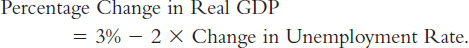
286
If the unemployment rate remains the same, real GDP grows by about 3 percent; this normal growth in the production of goods and services is due to growth in the labor force, capital accumulation, and technological progress. In addition, for every percentage point the unemployment rate rises, real GDP growth typically falls by 2 percent. Hence, if the unemployment rate rises from 5 to 7 percent, then real GDP growth would be

In this case, Okun’s law says that GDP would fall by 1 percent, indicating that the economy is in a recession.
Okun’s law is a reminder that the forces that govern the short-run business cycle are very different from those that shape long-run economic growth. As we saw in Chapter 8 and Chapter 9, long-run growth in GDP is determined primarily by technological progress. The long-run trend leading to higher standards of living from generation to generation is not associated with any long-run trend in the rate of unemployment. By contrast, short-run movements in GDP are highly correlated with the utilization of the economy’s labor force. The declines in the production of goods and services that occur during recessions are always associated with increases in joblessness.
287
Leading Economic Indicators
Many economists, particularly those working in business and government, are engaged in the task of forecasting short-run fluctuations in the economy. Business economists are interested in forecasting to help their companies plan for changes in the economic environment. Government economists are interested in forecasting for two reasons. First, the economic environment affects the government; for example, the state of the economy influences how much tax revenue the government collects. Second, the government can affect the economy through its use of monetary and fiscal policy. Economic forecasts are, therefore, an input into policy planning.
One way that economists arrive at their forecasts is by looking at leading indicators, which are variables that tend to fluctuate in advance of the overall economy. Forecasts can differ in part because economists hold varying opinions about which leading indicators are most reliable.
Each month the Conference Board, a private economics research group, announces the index of leading economic indicators. This index includes ten data series that are often used to forecast changes in economic activity about six to nine months into the future. Here is a list of the series:
Average weekly hours in manufacturing. Because businesses often adjust the work hours of existing employees before making new hires or laying off workers, average weekly hours is a leading indicator of employment changes. A longer workweek indicates that firms are asking their employees to work long hours because they are experiencing strong demand for their products; thus, it indicates that firms are likely to increase hiring and production in the future. A shorter workweek indicates weak demand, suggesting that firms are more likely to lay off workers and cut back production.
Average weekly initial claims for unemployment insurance. The number of people making new claims on the unemployment-insurance system is one of the most quickly available indicators of conditions in the labor market. This series is inverted in computing the index of leading indicators, so that an increase in the series lowers the index. An increase in the number of people making new claims for unemployment insurance indicates that firms are laying off workers and cutting back production; these layoffs and cutbacks will soon show up in data on employment and production.
Manufacturers’ new orders for consumer goods and materials. This indicator is a direct measure of the demand for consumer goods that firms are experiencing. Because an increase in orders depletes a firm’s inventories, this statistic typically predicts subsequent increases in production and employment.
288
Manufacturers’ new orders for nondefense capital goods, excluding aircraft. This series is the counterpart to the previous one, but for investment goods rather than consumer goods. When firms experience increased orders, they ramp up production and employment. Aircraft orders are excluded because they are often placed so far in advance of production that these orders contain little information about near-term economic activity.
ISM new orders index. This index, which comes from the Institute for Supply Management, is a third indicator of new orders. It is based on the number of companies reporting increased orders minus the number reporting decreased orders. Unlike the previous two indicators, this one measures the proportion of companies that report rising orders and thus shows whether a change is broadly based. When many firms experience increased orders, higher production and employment will likely soon follow.
Building permits for new private housing units. Construction of new buildings is part of investment—a particularly volatile component of GDP. An increase in building permits means that planned construction is increasing, which indicates a rise in overall economic activity.
Index of stock prices. The stock market reflects expectations about future economic conditions because stock market investors bid up prices when they expect companies to be profitable. An increase in stock prices indicates that investors expect the economy to grow rapidly; a decrease in stock prices indicates that investors expect an economic slowdown.
Leading Credit Index. This component is itself a composite of six financial indicators, such as investor sentiment (based on a survey of stock-market investors) and lending conditions (based on a survey of bank loan officers). When credit conditions are adverse, consumers and businesses find it harder to get the financing they need to make purchases. Thus, deterioration of credit conditions predicts a decline in spending, production, and employment. This index was added to the leading indicators only recently. The financial crisis of 2008–2009 and the subsequent deep recession highlighted the importance of credit conditions for economic activity.
Interest rate spread: the yield on 10-year Treasury bonds minus the federal funds rate. This spread, sometimes called the slope of the yield curve, reflects the market’s expectation about future interest rates, which in turn reflect the condition of the economy. A large spread means that interest rates are expected to rise, which typically occurs when economic activity increases.
Average consumer expectations for business and economic conditions. This is a direct measure of expectations, based on two different surveys of households (one conducted by the University of Michigan and one conducted by the Conference Board). Increased optimism about future economic conditions among consumers suggests increased consumer demand for goods and services, which in turn will encourage businesses to expand production and employment to meet the demand.
289
The index of leading indicators is far from a precise forecast of the future, as short-run economic fluctuations are largely unpredictable. Nonetheless, the index is a useful input into planning by both businesses and the government.