11.2 The Money Market and the LM Curve
The LM curve plots the relationship between the interest rate and the level of income that arises in the market for money balances. To understand this relationship, we begin by looking at a theory of the interest rate called the theory of liquidity preference.
The Theory of Liquidity Preference
In his classic work The General Theory, Keynes offered his view of how the interest rate is determined in the short run. His explanation is called the theory of liquidity preference because it posits that the interest rate adjusts to balance the supply and demand for the economy’s most liquid asset—
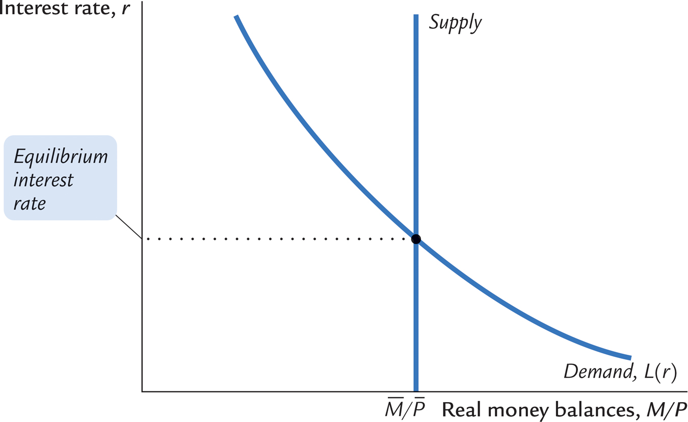
To develop this theory, we begin with the supply of real money balances. If M stands for the supply of money and P stands for the price level, then M/P is the supply of real money balances. The theory of liquidity preference assumes there is a fixed supply of real money balances. That is,

The money supply M is an exogenous policy variable chosen by a central bank, such as the Federal Reserve. The price level P is also an exogenous variable in this model. (We take the price level as given because the IS–LM model—

328
Next, consider the demand for real money balances. The theory of liquidity preference posits that the interest rate is one determinant of how much money people choose to hold. The underlying reason is that the interest rate is the opportunity cost of holding money: it is what you forgo by holding some of your assets as money, which does not bear interest, instead of as interest-
(M/P)d = L(r),
where the function L( ) shows that the quantity of money demanded depends on the interest rate. The demand curve in Figure 11-9 slopes downward because higher interest rates reduce the quantity of real money balances demanded.8
According to the theory of liquidity preference, the supply and demand for real money balances determine what interest rate prevails in the economy. That is, the interest rate adjusts to equilibrate the money market. As the figure shows, at the equilibrium interest rate, the quantity of real money balances demanded equals the quantity supplied.
329
How does the interest rate get to this equilibrium of money supply and money demand? The adjustment occurs because whenever the money market is not in equilibrium, people try to adjust their portfolios of assets and, in the process, alter the interest rate. For instance, if the interest rate is above the equilibrium level, the quantity of real money balances supplied exceeds the quantity demanded. Individuals holding the excess supply of money try to convert some of their non-
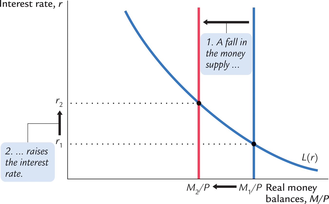
Now that we have seen how the interest rate is determined, we can use the theory of liquidity preference to show how the interest rate responds to changes in the supply of money. Suppose, for instance, that the Fed suddenly decreases the money supply. A fall in M reduces M/P because P is fixed in the model. The supply of real money balances shifts to the left, as in Figure 11-10. The equilibrium interest rate rises from r1 to r2, and the higher interest rate makes people satisfied to hold the smaller quantity of real money balances. The opposite would occur if the Fed had suddenly increased the money supply. Thus, according to the theory of liquidity preference, a decrease in the money supply raises the interest rate, and an increase in the money supply lowers the interest rate.

330
CASE STUDY
Does a Monetary Tightening Raise or LowerInterest Rates?
How does a tightening of monetary policy influence nominal interest rates? According to the theories we have been developing, the answer depends on the time horizon. Our analysis of the Fisher effect in Chapter 5 suggests that, in the long run when prices are flexible, a reduction in money growth would lower inflation, and this in turn would lead to lower nominal interest rates. Yet the theory of liquidity preference predicts that, in the short run when prices are sticky, anti-
Both conclusions are consistent with experience. A good illustration occurred during the early 1980s, when the U.S. economy saw the largest and quickest reduction in inflation in recent history.
Here’s the background: By the late 1970s, inflation in the U.S. economy had reached the double-
Let’s look at what happened to nominal interest rates. If we look at the period immediately after the October 1979 announcement of tighter monetary policy, we see a fall in real money balances and a rise in the interest rate—
This episode illustrates a general lesson: to understand the link between monetary policy and nominal interest rates, we need to keep in mind both the theory of liquidity preference and the Fisher effect. A monetary tightening leads to higher nominal interest rates in the short run and lower nominal interest rates in the long run. 
Income, Money Demand, and the LM Curve
Having developed the theory of liquidity preference as an explanation for how the interest rate is determined, we can now use the theory to derive the LM curve. We begin by considering the following question: How does a change in the economy’s level of income Y affect the market for real money balances? The answer (which should be familiar from Chapter 5) is that the level of income affects the demand for money. When income is high, expenditure is high, so people engage in more transactions that require the use of money. Thus, greater income implies greater money demand. We can express these ideas by writing the money demand function as
331
(M/P)d = L(r, Y).
The quantity of real money balances demanded is negatively related to the interest rate and positively related to income.
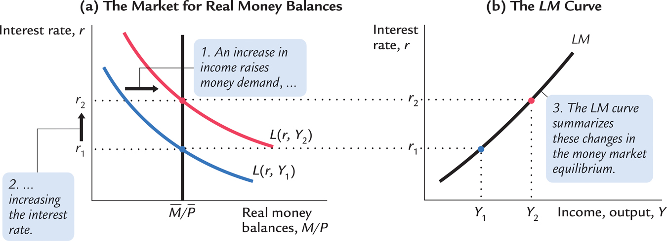
Using the theory of liquidity preference, we can figure out what happens to the equilibrium interest rate when the level of income changes. For example, consider what happens in Figure 11-11 when income increases from Y1 to Y2. As panel (a) illustrates, this increase in income shifts the money demand curve to the right. With the supply of real money balances unchanged, the interest rate must rise from r1 to r2 to equilibrate the money market. Therefore, according to the theory of liquidity preference, higher income leads to a higher interest rate.

The LM curve shown in panel (b) of Figure 11-11 summarizes this relationship between the level of income and the interest rate. Each point on the LM curve represents equilibrium in the money market, and the curve illustrates how the equilibrium interest rate depends on the level of income. The higher the level of income, the higher the demand for real money balances, and the higher the equilibrium interest rate. For this reason, the LM curve slopes upward.
332
How Monetary Policy Shifts the LM Curve
The LM curve tells us the interest rate that equilibrates the money market at any level of income. Yet, as we saw earlier, the equilibrium interest rate also depends on the supply of real money balances M/P. This means that the LM curve is drawn for a given supply of real money balances. If real money balances change—
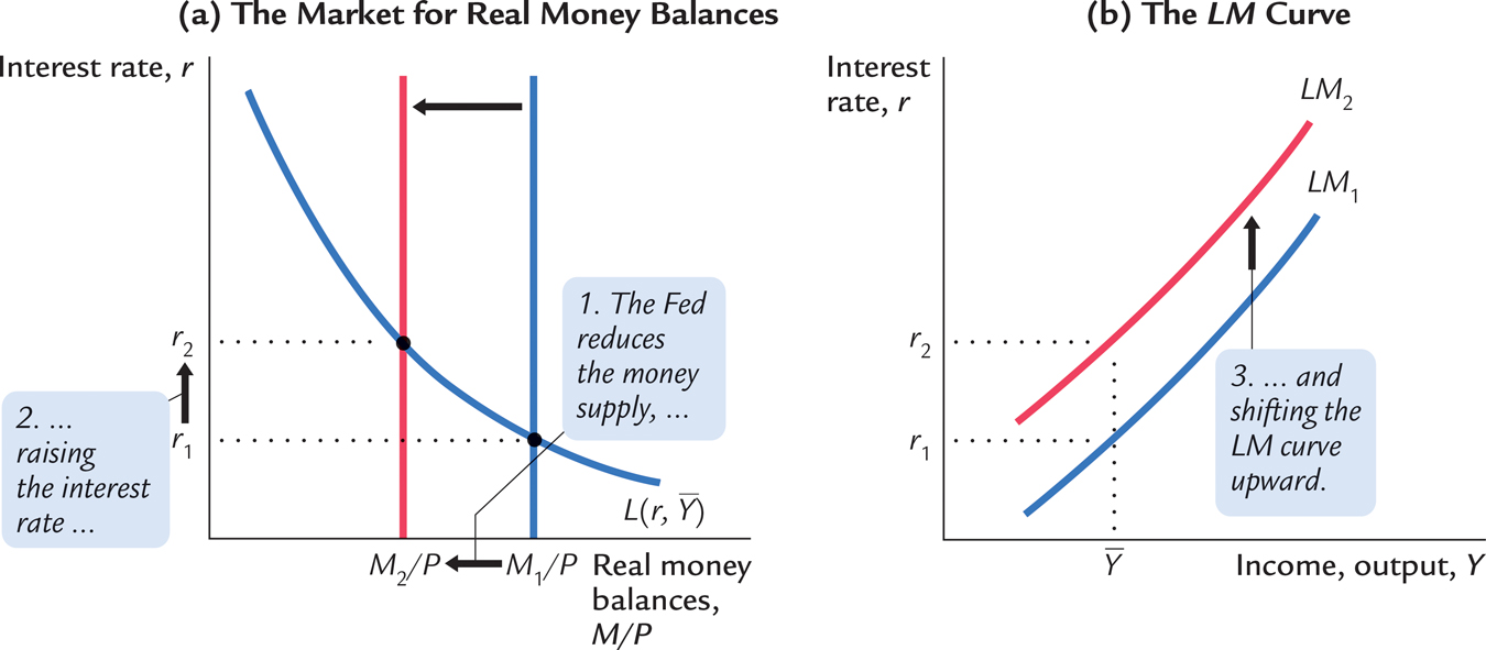
We can use the theory of liquidity preference to understand how monetary policy shifts the LM curve. Suppose that the Fed decreases the money supply from M1 to M2, which causes the supply of real money balances to fall from M1/P to M2/P. Figure 11-12 shows what happens. Holding constant the amount of income and thus the demand curve for real money balances, we see that a reduction in the supply of real money balances raises the interest rate that equilibrates the money market. Hence, a decrease in the money supply shifts the LM curve upward.

 , a reduction in the money supply raises the interest rate that equilibrates the money market. Therefore, the LM curve in panel (b) shifts upward.
In summary, the LM curve shows the combinations of the interest rate and the level of income that are consistent with equilibrium in the market for real money balances. The LM curve is drawn for a given supply of real money balances. Decreases in the supply of real money balances shift the LM curve upward. Increases in the supply of real money balances shift the LM curve downward.
333