In this section, we construct the Mundell–Fleming model; and in the following sections, we use the model to examine the impact of various policies. As you will see, the Mundell–Fleming model is built from components we have used in previous chapters. But these pieces are put together in a new way to address a new set of questions.

Let’s begin with the assumption of a small open economy with perfect capital mobility. As we saw in Chapter 6, this assumption means that the interest rate in this economy r is determined by the world interest rate r*. Mathematically, we write this assumption as

r = r*.

This world interest rate is assumed to be exogenously fixed because the economy is sufficiently small relative to the world economy that it can borrow or lend as much as it wants in world financial markets without affecting the world interest rate.

Although the idea of perfect capital mobility is expressed with a simple equation, it is important not to lose sight of the sophisticated process that this equation represents. Imagine that some event occurred that would normally raise the interest rate (such as a decline in domestic saving). In a small open economy, the domestic interest rate might rise by a little bit for a short time, but as soon as it did, foreigners would see the higher interest rate and start lending to this country (by, for instance, buying this country’s bonds). The capital inflow would drive the domestic interest rate back toward r*. Similarly, if any event started to drive the domestic interest rate downward, capital would flow out of the country to earn a higher return abroad, and this capital outflow would drive the domestic interest rate back up to r*. Hence, the r = r* equation represents the assumption that the international flow of capital is rapid enough to keep the domestic interest rate equal to the world interest rate.

370

The Mundell–Fleming model describes the market for goods and services much as the IS–LM model does, but it adds a new term for net exports. In particular, the goods market is represented with the following equation:

Y = C(Y − T) + I(r) + G + NX(e).

This equation states that aggregate income Y is the sum of consumption C, investment I, government purchases G, and net exports NX. Consumption depends positively on disposable income Y − T. Investment depends negatively on the interest rate. Net exports depend negatively on the exchange rate e. As before, we define the exchange rate e as the amount of foreign currency per unit of domestic currency—for example, e might be 100 yen per dollar.

You may recall that in Chapter 6 we related net exports to the real exchange rate (the relative price of goods at home and abroad) rather than the nominal exchange rate (the relative price of domestic and foreign currencies). If e is the nominal exchange rate, then the real exchange rate ε equals eP/P*, where P is the domestic price level and P* is the foreign price level. The Mundell–Fleming model, however, assumes that the price levels at home and abroad are fixed, so the real exchange rate is proportional to the nominal exchange rate. That is, when the domestic currency appreciates and the nominal exchange rate rises (from, say, 100 to 120 yen per dollar), the real exchange rate rises as well; thus, foreign goods become cheaper compared to domestic goods, and this causes exports to fall and imports to rise.

The goods market equilibrium condition above has two financial variables that affect expenditure on goods and services (the interest rate and the exchange rate), but we can simplify matters by using the assumption of perfect capital mobility, r = r*:

Y = C(Y − T) + I(r*) + G + NX(e).

Let’s call this the IS* equation. (The asterisk reminds us that the equation holds the interest rate constant at the world interest rate r*.) We can illustrate this equation on a graph in which income is on the horizontal axis and the exchange rate is on the vertical axis. This curve is shown in panel (c) of Figure 13-1.

The IS* curve slopes downward because a higher exchange rate reduces net exports, which in turn lowers aggregate income. To show how this works, the other panels of Figure 13-1 combine the net-exports schedule and the Keynesian cross to derive the IS* curve. In panel (a), an increase in the exchange rate from e₁ to e₂ lowers net exports from NX(e₁) to NX(e₂). In panel (b), the reduction in net exports shifts the planned-expenditure schedule downward and thus lowers income from Y₁ to Y₂. The IS* curve summarizes this relationship between the exchange rate e and income Y.

The Mundell–Fleming model represents the money market with an equation that should be familiar from the IS–LM model:

M/P = L(r, Y).

371

This equation states that the supply of real money balances M/P equals the demand L(r, Y). The demand for real balances depends negatively on the interest rate and positively on income. The money supply M is an exogenous variable controlled by the central bank, and because the Mundell–Fleming model is designed to analyze short-run fluctuations, the price level P is also assumed to be exogenously fixed.

Once again, we add the assumption that the domestic interest rate equals the world interest rate, so r = r*:

M/P = L(r*, Y).

Let’s call this the LM* equation. We can represent it graphically with a vertical line, as in panel (b) of Figure 13-2. The LM* curve is vertical because the exchange rate does not enter into the LM* equation. Given the world interest rate, the LM* equation determines aggregate income, regardless of the exchange rate. Figure 13-2 shows how the LM* curve arises from the world interest rate and the LM curve, which relates the interest rate and income.

372

According to the Mundell–Fleming model, a small open economy with perfect capital mobility can be described by two equations:

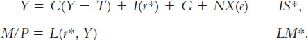
The first equation describes equilibrium in the goods market; the second describes equilibrium in the money market. The exogenous variables are fiscal policy G and T, monetary policy M, the price level P, and the world interest rate r*. The endogenous variables are income Y and the exchange rate e.

373

Figure 13-3 illustrates these two relationships. The equilibrium for the economy is found where the IS* curve and the LM* curve intersect. This intersection shows the exchange rate and the level of income at which the goods market and the money market are both in equilibrium. With this diagram, we can use the Mundell–Fleming model to show how aggregate income Y and the exchange rate e respond to changes in policy.