So far we have used the Mundell–Fleming model to study the small open economy in the short run when the price level is fixed. We now consider what happens when the price level changes. Doing so will show how the Mundell–Fleming model provides a theory of the aggregate demand curve in a small open economy. It will also show how this short-run model relates to the long-run model of the open economy we examined in Chapter 6.

Because we now want to consider changes in the price level, the nominal and real exchange rates in the economy will no longer be moving in tandem. Thus, we must distinguish between these two variables. The nominal exchange rate is e and the real exchange rate is ε, which equals eP/P*, as you should recall from Chapter 6. We can write the Mundell–Fleming model as

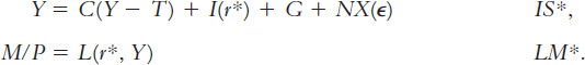
These equations should be familiar by now. The first equation describes the IS* curve; and the second describes the LM* curve. Note that net exports depend on the real exchange rate.

Figure 13-13 shows what happens when the price level falls. Because a lower price level raises the level of real money balances, the LM* curve shifts to the right, as in panel (a). The real exchange rate falls, and the equilibrium level of income rises. The aggregate demand curve summarizes this negative relationship between the price level and the level of income, as shown in panel (b).

Thus, just as the IS-LM model explains the aggregate demand curve in a closed economy, the Mundell–Fleming model explains the aggregate demand curve for a small open economy. In both cases, the aggregate demand curve shows the set of equilibria in the goods and money markets that arise as the price level varies. And in both cases, anything that changes equilibrium income, other than a change in the price level, shifts the aggregate demand curve. Policies and events that raise income for a given price level shift the aggregate demand curve to the right; policies and events that lower income for a given price level shift the aggregate demand curve to the left.

396

We can use this diagram to show how the short-run model in this chapter is related to the long-run model in Chapter 6. Figure 13-14 shows the short-run and long-run equilibria. In both panels of the figure, point K describes the short-run equilibrium because it assumes a fixed price level. At this equilibrium, the demand for goods and services is too low to keep the economy producing at its natural level. Over time, low demand causes the price level to fall. The fall in the price level raises real money balances, shifting the LM* curve to the right. The real exchange rate depreciates, so net exports rise. Eventually, the economy reaches point C, the long-run equilibrium. The speed of transition between the short-run and long-run equilibria depends on how quickly the price level adjusts to restore the economy to the natural level of output.

397

The levels of income at point K and point C are both of interest. Our central concern in this chapter has been how policy influences point K, the short-run equilibrium. In Chapter 6 we examined the determinants of point C, the long-run equilibrium. Whenever policymakers consider any change in policy, they need to consider both the short-run and long-run effects of their decision.

398