In this section we consider the determinants of residential investment. We begin by presenting a simple model of the housing market. Residential investment includes the purchase of new housing both by people who plan to live in it themselves and by landlords who plan to rent it to others. To keep things simple, however, it is useful to imagine that all housing is owner-occupied.

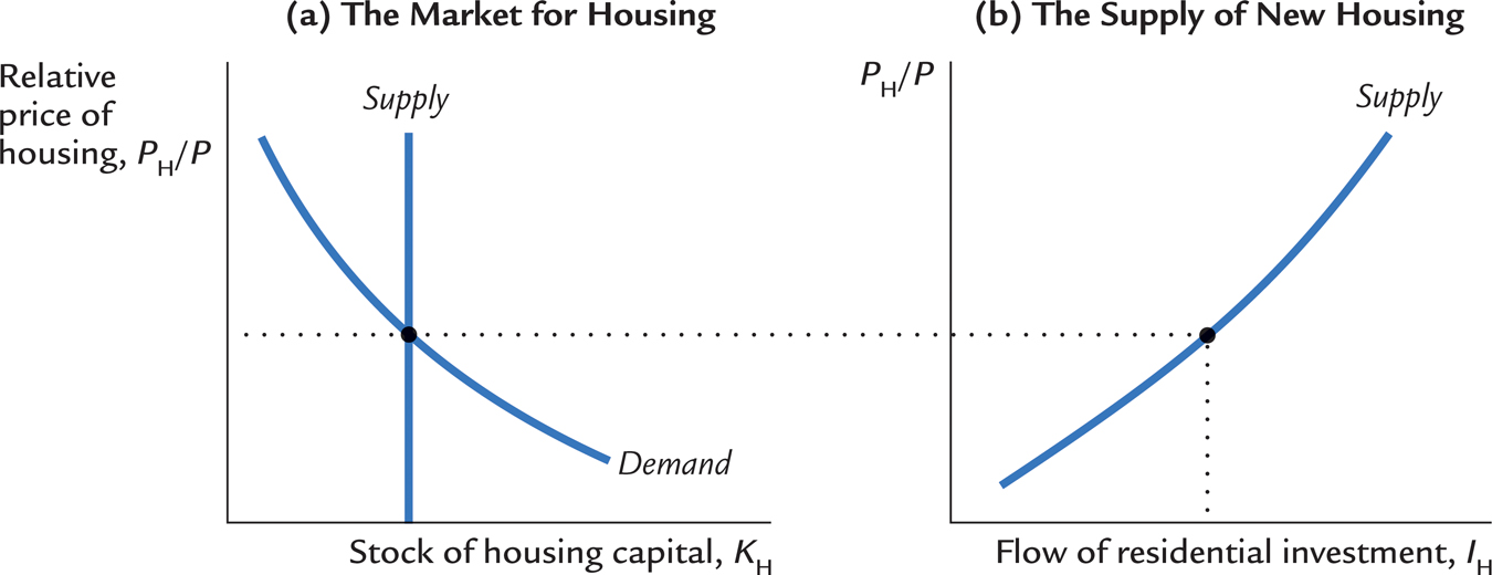
There are two parts to the model. First, the market for the existing stock of houses determines the equilibrium housing price. Second, the housing price determines the flow of residential investment.

Panel (a) of Figure 17-5 shows how the relative price of housing P_H/P is determined by the supply and demand for the existing stock of houses. At any point in time, the supply of houses is fixed. We represent this stock with a vertical supply curve. The demand curve for houses slopes downward because high prices cause people to live in smaller houses, to share residences, or sometimes even to become homeless. The price of housing adjusts to equilibrate supply and demand.

Panel (b) of Figure 17-5 shows how the relative price of housing determines the supply of new houses. Construction firms buy materials and hire labor to build houses and then sell the houses at the market price. Their costs depend on the overall price level P (which reflects the cost of wood, bricks, plaster, etc.), and their revenue depends on the price of houses P_H. The higher the relative price of housing, the greater the incentive to build houses and the more houses are built. The flow of new houses—residential investment—therefore depends on the equilibrium price set in the market for existing houses.

523

This model of residential investment is similar to the q theory of business fixed investment. According to the q theory, business fixed investment depends on the market price of installed capital relative to its replacement cost; this relative price, in turn, depends on the expected profits from owning installed capital. According to this model of the housing market, residential investment depends on the relative price of housing. The relative price of housing, in turn, depends on the demand for housing, which depends on the imputed rent that individuals expect to receive from their housing. Hence, the relative price of housing plays much the same role for residential investment as Tobin’s q does for business fixed investment.

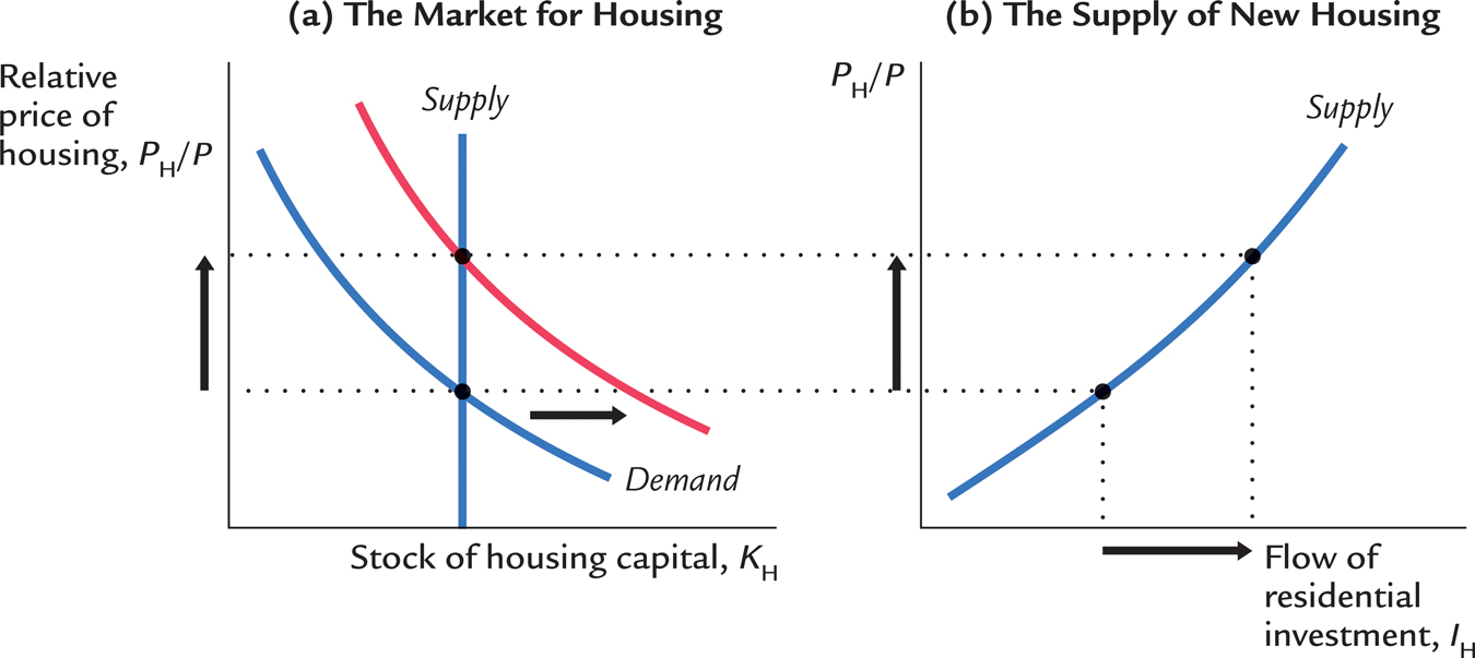
When the demand for housing shifts, the equilibrium price of housing changes, and this change in turn affects residential investment. The demand curve for housing can shift for various reasons. An economic boom raises national income and therefore the demand for housing. A large increase in the population, perhaps because of immigration, also raises the demand for housing. Panel (a) of Figure 17-6 shows that an expansionary shift in demand raises the equilibrium price. Panel (b) shows that the increase in the housing price increases residential investment.

524

One important determinant of housing demand is the real interest rate. Many people take out loans—mortgages—to buy their homes; the interest rate is the cost of the loan. Even the few people who do not have to borrow to purchase a home will respond to the interest rate because the interest rate is the opportunity cost of holding their wealth in housing rather than putting it in a bank. A reduction in the interest rate therefore raises housing demand, housing prices, and residential investment.

Another important determinant of housing demand is credit availability. When it is easy to get a loan, more households buy their own homes, and they buy larger ones than they otherwise might, thus increasing the demand for housing. When credit conditions become tight, fewer people buy their own homes or trade up to larger ones, and the demand for housing falls.

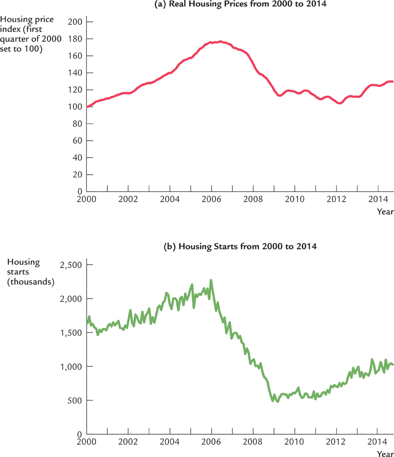
An example of this phenomenon occurred during the first decade of the twenty-first century. Early in this decade, interest rates were low, and mortgages were easy to come by. Many households with questionable credit histories—called subprime borrowers—were able to get mortgages with small down payments. Not surprisingly, the housing market boomed. Housing prices rose, and residential investment was strong. A few years later, however, it became clear that the situation had gotten out of hand, as many of these subprime borrowers could not keep up with their mortgage payments. When interest rates rose and credit conditions tightened, housing demand and housing prices started to fall. Figure 17-7 illustrates the movement of housing prices and housing starts during this period. When the housing market turned down in 2007 and 2008, the result was a significant downturn in the overall economy, which is discussed in a Case Study in Chapter 12.

525

526