2.1 Measuring the Value of Economic Activity: Gross Domestic Product
Gross domestic product, or GDP, is often considered the best measure of how well an economy is performing. In the United States, this statistic is computed every three months by the Bureau of Economic Analysis, a part of the U.S. Department of Commerce, from a large number of primary data sources. These primary sources include both (1) administrative data, which are byproducts of government functions such as tax collection, education programs, defense, and regulation, and (2) statistical data, which come from government surveys of, for example, retail establishments, manufacturing firms, and farms. The purpose of GDP is to summarize all these data with a single number representing the dollar value of economic activity in a given period of time.
There are two ways to view this statistic. One way to view GDP is as the total income of everyone in the economy; another way is as the total expenditure on the economy’s output of goods and services. From either viewpoint, it is clear why GDP is a gauge of economic performance. GDP measures something people care about—
How can GDP measure both the economy’s income and its expenditure on output? The reason is that these two quantities are really the same: for the economy as a whole, income must equal expenditure. That fact, in turn, follows from an even more fundamental one: because every transaction has a buyer and a seller, every dollar of expenditure by a buyer must become a dollar of income to a seller. When Jack paints Jill’s house for $10,000, that $10,000 is income to Jack and expenditure by Jill. The transaction contributes $10,000 to GDP, regardless of whether we are adding up all income or all expenditure.
To understand the meaning of GDP more fully, we turn to national income accounting, the system used to measure GDP and many related statistics.
Income, Expenditure, and the Circular Flow
Imagine an economy that produces a single good, bread, from a single input, labor. Figure 2-1 illustrates all the economic transactions that occur between households and firms in this economy.

19
The inner loop in Figure 2-1 represents the flows of bread and labor. The households sell their labor to the firms. The firms use the labor of their workers to produce bread, which the firms in turn sell to the households. Hence, labor flows from households to firms, and bread flows from firms to households.
The outer loop in Figure 2-1 represents the corresponding flow of dollars. The households buy bread from the firms. The firms use some of the revenue from these sales to pay the wages of their workers, and the remainder is the profit belonging to the owners of the firms (who themselves are part of the household sector). Hence, expenditure on bread flows from households to firms, and income in the form of wages and profit flows from firms to households.
GDP measures the flow of dollars in this economy. We can compute it in two ways. GDP is the total income from the production of bread, which equals the sum of wages and profit—
20
These two ways of computing GDP must be equal because, by the rules of accounting, the expenditure of buyers on products is income to the sellers of those products. Every transaction that affects expenditure must affect income, and every transaction that affects income must affect expenditure. For example, suppose that a firm produces and sells one more loaf of bread to a household. Clearly this transaction raises total expenditure on bread, but it also has an equal effect on total income. If the firm produces the extra loaf without hiring any more labor (such as by making the production process more efficient), then profit increases. If the firm produces the extra loaf by hiring more labor, then wages increase. In both cases, expenditure and income increase equally.
FYI
Stocks and Flows
Many economic variables measure a quantity of something—
A bathtub, shown in Figure 2-2, is the classic example used to illustrate stocks and flows. The amount of water in the tub is a stock: it is the quantity of water in the tub at a given point in time. The amount of water coming out of the faucet is a flow: it is the quantity of water being added to the tub per unit of time. Note that we measure stocks and flows in different units. We say that the bathtub contains 50 gallons of water but that water is coming out of the faucet at 5 gallons per minute.

GDP is probably the most important flow variable in economics: it tells us how many dollars are flowing around the economy’s circular flow per unit of time. When someone says that the U.S. GDP is $17 trillion, this means that it is $17 trillion per year. (Equivalently, we could say that U.S. GDP is $539,000 per second.)
Stocks and flows are often related. In the bathtub example, these relationships are clear. The stock of water in the tub represents the accumulation of the flow out of the faucet, and the flow of water represents the change in the stock. When building theories to explain economic variables, it is often useful to determine whether the variables are stocks or flows and whether any relationships link them.
Here are some examples of related stocks and flows that we study in future chapters:
A person’s wealth is a stock; his income and expenditure are flows.
The number of unemployed people is a stock; the number of people losing their jobs is a flow.
The amount of capital in the economy is a stock; the amount of investment is a flow.
The government debt is a stock; the government budget deficit is a flow.
21
Rules for Computing GDP
In an economy that produces only bread, we can compute GDP by adding up the total expenditure on bread. Real economies, however, include the production and sale of a vast number of goods and services. To compute GDP for such a complex economy, it will be helpful to have a more precise definition: Gross domestic product (GDP) is the market value of all final goods and services produced within an economy in a given period of time. To see how this definition is applied, let’s discuss some of the rules that economists follow in constructing this statistic.
Adding Apples and Oranges The U.S. economy produces many different goods and services—
Suppose, for example, that the economy produces four apples and three oranges. How do we compute GDP? We could simply add apples and oranges and conclude that GDP equals seven pieces of fruit. But this makes sense only if we think apples and oranges have equal value, which is generally not true. (This would be even clearer if the economy produces four watermelons and three grapes.)
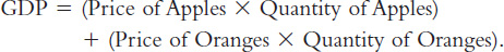
To compute the total value of different goods and services, the national income accounts use market prices because these prices reflect how much people are willing to pay for a good or service. Thus, if apples cost $0.50 each and oranges cost $1.00 each, GDP would be
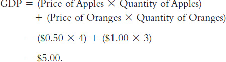
GDP equals $5.00—
Used Goods When the Topps Company makes a pack of baseball cards and sells it for $2, that $2 is added to the nation’s GDP. But when a collector sells a rare Mickey Mantle card to another collector for $500, that $500 is not part of GDP. GDP measures the value of currently produced goods and services. The sale of the Mickey Mantle card reflects the transfer of an asset, not an addition to the economy’s income. Thus, the sale of used goods is not included as part of GDP.
The Treatment of Inventories Imagine that a bakery hires workers to produce more bread, pays their wages, and then fails to sell the additional bread. How does this transaction affect GDP?
The answer depends on what happens to the unsold bread. Let’s first suppose that the bread spoils. In this case, the firm has paid more in wages but has not received any additional revenue, so the firm’s profit is reduced by the amount that wages have increased. Total expenditure in the economy hasn’t changed because no one buys the bread. Total income hasn’t changed either—
22
Now suppose, instead, that the bread is put into inventory (perhaps as frozen dough) to be sold later. In this case, the national income accounts treat the transaction differently. The owners of the firm are assumed to have “purchased” the bread for the firm’s inventory, and the firm’s profit is not reduced by the additional wages it has paid. Because the higher wages paid to the firm’s workers raise total income, and the greater spending by the firm’s owners on inventory raises total expenditure, the economy’s GDP rises.
What happens later when the firm sells the bread out of inventory? This case is much like the sale of a used good. There is spending by bread consumers, but there is inventory disinvestment by the firm. This negative spending by the firm offsets the positive spending by consumers, so the sale out of inventory does not affect GDP.
The general rule is that when a firm increases its inventory of goods, this investment in inventory is counted as an expenditure by the firm owners. Thus, production for inventory increases GDP just as much as does production for final sale. A sale out of inventory, however, is a combination of positive spending (the purchase) and negative spending (inventory disinvestment), so it does not influence GDP. This treatment of inventories ensures that GDP reflects the economy’s current production of goods and services.
Intermediate Goods and Value Added Many goods are produced in stages: raw materials are processed into intermediate goods by one firm and then sold to another firm for final processing. How should we treat such products when computing GDP? For example, suppose a cattle rancher sells one-
The answer is that GDP includes only the value of final goods. Thus, the hamburger is included in GDP but the meat is not: GDP increases by $3, not by $4. The reason is that the value of intermediate goods is already included as part of the market price of the final goods in which they are used. To add the intermediate goods to the final goods would be double counting—
One way to compute the value of all final goods and services is to sum the value added at each stage of production. The value added of a firm equals the value of the firm’s output less the value of the intermediate goods that the firm purchases. In the case of the hamburger, the value added of the rancher is $1 (assuming that the rancher bought no intermediate goods), and the value added of McDonald’s is $3 – $1, or $2. Total value added is $1 + $2, which equals $3. For the economy as a whole, the sum of all value added must equal the value of all final goods and services. Hence, GDP is also the total value added of all firms in the economy.
Housing Services and Other Imputations Although most goods and services are valued at their market prices when computing GDP, some are not sold in the marketplace and therefore do not have market prices. If GDP is to include the value of these goods and services, we must use an estimate of their value. Such an estimate is called an imputed value.
23
Imputations are especially important for determining the value of housing. A person who rents a house is buying housing services and providing income for the landlord; the rent is part of GDP, both as expenditure by the renter and as income for the landlord. Many people, however, own their homes. Although they do not pay rent to a landlord, they are enjoying housing services similar to those that renters purchase. To take account of the housing services enjoyed by homeowners, GDP includes the “rent” that these homeowners “pay” to themselves. Of course, homeowners do not in fact pay themselves this rent. The Department of Commerce estimates what the market rent for a house would be if it were rented and includes that imputed rent as part of GDP. This imputed rent is included both in the homeowner’s expenditure and in the homeowner’s income.
Imputations also arise in valuing government services. For example, police officers, firefighters, and senators provide services to the public. Assigning a value to these services is difficult because they are not sold in a marketplace and therefore do not have a market price. The national income accounts include these services in GDP by valuing them at their cost. That is, the wages of these public servants are used as a measure of the value of their output.
In many cases, an imputation is called for in principle but, to keep things simple, is not made in practice. Because GDP includes the imputed rent on owner-
Finally, no imputation is made for the value of goods and services sold in the underground economy. The underground economy is the part of the economy that people hide from the government either because they wish to evade taxation or because the activity is illegal. Examples include domestic workers paid “off the books” and the illegal drug trade. The size of the underground economy varies widely from country to country. In the United States, the underground economy is estimated to be less than 10 percent of the official economy, whereas in some developing nations, such as Thailand, Nigeria, and Bolivia, the underground economy is more than half as large as the official one.
Because the imputations necessary for computing GDP are only approximate, and because the value of many goods and services is left out altogether, GDP is an imperfect measure of economic activity. These imperfections are most problematic when comparing standards of living across countries. Yet as long as the magnitude of these imperfections remains fairly constant over time, GDP is useful for comparing economic activity from year to year.
Real GDP Versus Nominal GDP
Economists use the rules just described to compute GDP, which values the economy’s total output of goods and services. But is GDP a good measure of economic well-
24
Economists call the value of goods and services measured at current prices nominal GDP. Notice that nominal GDP can increase either because prices rise or because quantities rise.
It is easy to see that GDP computed this way is not a good gauge of economic well-
A better measure of economic well-
To see how real GDP is computed, imagine we want to compare output in 2014 with output in subsequent years for our apple-

Similarly, real GDP in 2015 would be

And real GDP in 2016 would be

Notice that 2014 prices are used to compute real GDP for all three years. Because the prices are held constant, real GDP varies from year to year only if the quantities produced vary. Because a society’s ability to provide economic satisfaction for its members ultimately depends on the quantities of goods and services produced, real GDP provides a better measure of economic well-
25
The GDP Deflator
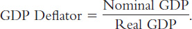
From nominal GDP and real GDP we can compute a third statistic: the GDP deflator. The GDP deflator, also called the implicit price deflator for GDP, is the ratio of nominal GDP to real GDP:
The GDP deflator reflects what’s happening to the overall level of prices in the economy.
To better understand this, consider again an economy with only one good, bread. If P is the price of bread and Q is the quantity sold, then nominal GDP is the total number of dollars spent on bread in that year, P × Q. Real GDP is the number of loaves of bread produced in that year times the price of bread in some base year, Pbase × Q. The GDP deflator is the price of bread in that year relative to the price of bread in the base year, P/Pbase.
The definition of the GDP deflator allows us to separate nominal GDP into two parts: one part measures quantities (real GDP) and the other measures prices (the GDP deflator). That is,
Nominal GDP = Real GDP × GDP Deflator.
Nominal GDP measures the current dollar value of the output of the economy. Real GDP measures output valued at constant prices. The GDP deflator measures the price of output relative to its price in the base year. We can also write this equation as
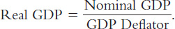
In this form, you can see how the deflator earns its name: it is used to deflate (that is, take inflation out of) nominal GDP to yield real GDP.
Chain-Weighted Measures of Real GDP
We have been discussing real GDP as if the prices used to compute this measure never change from their base-
To solve this problem, the Bureau of Economic Analysis used to periodically update the prices used to compute real GDP. About every five years, a new base year was chosen. The prices were then held fixed and used to measure year-
In 1995, the Bureau announced a new policy for dealing with changes in the base year. In particular, it now uses chain-
26
This new chain-
FYI
Two Arithmetic Tricks for Working with Percentage Changes
For manipulating many relationships in economics, there is an arithmetic trick that is useful to know: The percentage change of a product of two variables is approximately the sum of the percentage changes in each of the variables.
To see how this trick works, consider an example. Let P denote the GDP deflator and Y denote real GDP. Nominal GDP is P × Y. The trick states that
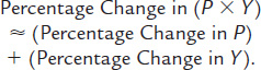
For instance, suppose that in one year, real GDP is 100 and the GDP deflator is 2; the next year, real GDP is 103 and the GDP deflator is 2.1. We can calculate that real GDP rose by 3 percent and that the GDP deflator rose by 5 percent. Nominal GDP rose from 200 the first year to 216.3 the second year, an increase of 8.15 percent. Notice that the growth in nominal GDP (8.15 percent) is approximately the sum of the growth in the GDP deflator (5 percent) and the growth in real GDP (3 percent).1
A second arithmetic trick follows as a corollary to the first: The percentage change of a ratio is approximately the percentage change in the numerator minus the percentage change in the denominator. Again, consider an example. Let Y denote GDP and L denote the population, so that Y/L is GDP per person. The second trick states that
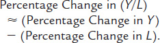
For instance, suppose that in the first year, Y is 100,000 and L is 100, so Y/L is 1,000; in the second year, Y is 110,000 and L is 103, so Y/L is 1,068. Notice that the growth in GDP per person (6.8 percent) is approximately the growth in income (10 percent) minus the growth in population (3 percent).
27
The Components of Expenditure
Economists and policymakers care not only about the economy’s total output of goods and services but also about the allocation of this output among alternative uses. The national income accounts divide GDP into four broad categories of spending:
Consumption (C)
Investment (I)
Government purchases (G)
Net exports (NX).
Thus, letting Y stand for GDP,
Y = C + I + G + NX.
GDP is the sum of consumption, investment, government purchases, and net exports. Each dollar of GDP falls into one of these categories. This equation is an identity—an equation that must hold because of the way the variables are defined. It is called the national income accounts identity.
Consumption consists of household expenditures on goods and services. Goods are tangible items, and they in turn are divided into durables and nondurables. Durable goods are goods that last a long time, such as cars and TVs. Nondurable goods are goods that last only a short time, such as food and clothing. Services include various intangible items that consumers buy, such as haircuts and doctor visits.
Investment consists of items bought for future use. Investment is divided into three subcategories: business fixed investment, residential fixed investment, and inventory investment. Business fixed investment, also called nonresidential fixed investment, is the purchase by firms of new structures, equipment, and intellectual property products. (Intellectual property products include software, research and development, and entertainment, literary, and artistic originals.) Residential investment is the purchase of new housing by households and landlords. Inventory investment is the increase in firms’ inventories of goods (if inventories are falling, inventory investment is negative).
Government purchases are the goods and services bought by federal, state, and local governments. This category includes such items as military equipment, highways, and the services provided by government workers. It does not include transfer payments to individuals, such as Social Security and welfare. Because transfer payments reallocate existing income and are not made in exchange for goods and services, they are not part of GDP.
The last category, net exports, accounts for trade with other countries. Net exports are the value of goods and services sold to other countries (exports) minus the value of goods and services that foreigners sell us (imports). Net exports are positive when the value of our exports is greater than the value of our imports and negative when the value of our imports is greater than the value of our exports. Net exports represent the net expenditure from abroad on our goods and services, which provides income for domestic producers.
28
FYI
What Is Investment?
Newcomers to macroeconomics are sometimes confused by how macroeconomists use familiar words in new and specific ways. One example is the term “investment.” The confusion arises because what looks like investment for an individual may not be investment for the economy as a whole. The general rule is that the economy’s investment does not include purchases that merely reallocate existing assets among different individuals. Investment, as macroeconomists use the term, creates a new physical asset, called capital, which can be used in future production.
Let’s consider some examples. Suppose we observe these two events:
Smith buys himself a 100-
year- old Victorian house. Jones builds herself a brand-
new contemporary house.
What is total investment here? Two houses, one house, or zero?
A macroeconomist seeing these two transactions counts only the Jones house as investment. Smith’s transaction has not created new housing for the economy; it has merely reallocated existing housing to Smith from the previous owner. By contrast, because Jones has added new housing to the economy, her new house is counted as investment.
Similarly, consider these two events:
Gates buys $5 million in IBM stock from Buffett on the New York Stock Exchange.
General Motors sells $10 million in stock to the public and uses the proceeds to build a new car factory.
Here, investment is $10 million. The first transaction reallocates ownership of shares in IBM from Buffett to Gates; the economy’s stock of capital is unchanged, so there is no investment as macroeconomists use the term. By contrast, because General Motors is using some of the economy’s output of goods and services to add to its stock of capital, its new factory is counted as investment.
CASE STUDY
GDP and Its Components
In 2013, the GDP of the United States totaled about $16.8 trillion. This number is so large that it is almost impossible to comprehend. We can make it easier to understand by dividing it by the 2013 U.S. population of 316 million. In this way, we obtain GDP per person—
How did this GDP get used? Table 2-1 shows that about two-

The average American bought $8,722 of goods imported from abroad and produced $7,149 of goods that were exported to other countries. Because the average American imported more than he exported, net exports were negative. Furthermore, because the average American earned less from selling to foreigners than he spent on foreign goods, he must have financed the difference by taking out loans from foreigners (or, equivalently, by selling them some of his assets). Thus, the average American borrowed $1,573 from abroad in 2013. 
29
Other Measures of Income
The national income accounts include other measures of income that differ slightly in definition from GDP. It is important to be aware of the various measures, because economists and the media often refer to them.
To see how the alternative measures of income relate to one another, we start with GDP and modify it in various ways. To obtain gross national product (GNP), we add to GDP receipts of factor income (wages, profit, and rent) from the rest of the world and subtract payments of factor income to the rest of the world:
GNP = GDP + Factor Payments from Abroad − Factor Payments to Abroad.
Whereas GDP measures the total income produced domestically, GNP measures the total income earned by nationals (residents of a nation). For instance, if a Japanese resident owns an apartment building in New York, the rental income he earns is part of U.S. GDP because it is earned in the United States. But because this rental income is a factor payment to abroad, it is not part of U.S. GNP. In the United States, factor payments from abroad and factor payments to abroad are similar in size—
30
To obtain net national product (NNP), we subtract from GNP the depreciation of capital—
NNP = GNP − Depreciation.
In the national income accounts, depreciation is called the consumption of fixed capital. It equals about 16 percent of GNP. Because the depreciation of capital is a cost of producing the output of the economy, subtracting depreciation shows the net result of economic activity.
Net national product is approximately equal to another measure called national income. The two differ by a small correction called the statistical discrepancy, which arises because different data sources may not be completely consistent.
National Income = NNP − Statistical Discrepancy.
National income measures how much everyone in the economy has earned.
The national income accounts divide national income into six components, depending on who earns the income. The six categories, and the percentage of national income paid in each category in 2013, are the following:
Compensation of employees (61%). The wages and fringe benefits earned by workers.
Proprietors’ income (9%). The income of noncorporate businesses, such as small farms, mom-
and- pop stores, and law partnerships. Rental income (4%). The income that landlords receive, including the imputed rent that homeowners “pay” to themselves, less expenses, such as depreciation.
Corporate profits (15%). The income of corporations after payments to their workers and creditors.
Net interest (3%). The interest domestic businesses pay minus the interest they receive, plus interest earned from foreigners.
Taxes on production and imports (8%). Certain taxes on businesses, such as sales taxes, less offsetting business subsidies. These taxes place a wedge between the price that consumers pay for a good and the price that firms receive.
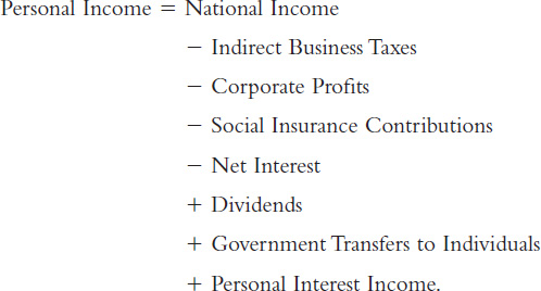
A series of adjustments take us from national income to personal income, the amount of income that households and noncorporate businesses receive. Four of these adjustments are most important. First, we subtract taxes on production and imports because these taxes never enter anyone’s income. Second, we reduce national income by the amount that corporations earn but do not pay out, either because the corporations are retaining earnings or because they are paying taxes to the government. This adjustment is made by subtracting corporate profits (which equal the sum of corporate taxes, dividends, and retained earnings) and adding back dividends. Third, we increase national income by the net amount the government pays out in transfer payments. This adjustment equals government transfers to individuals minus social insurance contributions paid to the government. Fourth, we adjust national income to include the interest that households earn rather than the interest that businesses pay. This adjustment is made by adding personal interest income and subtracting net interest. (The difference between personal interest and net interest arises in part because interest on the government debt is part of the interest that households earn but is not part of the interest that businesses pay out.) Thus,
31
Next, if we subtract personal taxes, we obtain disposable personal income:
Disposable Personal Income = Personal Income − Personal Taxes.
We are interested in disposable personal income because it is the amount households and noncorporate businesses have available to spend after satisfying their tax obligations to the government.
Seasonal Adjustment
Because real GDP and the other measures of income reflect how well the economy is performing, economists are interested in studying the quarter-
It is not surprising that real GDP follows a seasonal cycle. Some of these changes are attributable to changes in our ability to produce: for example, building homes is more difficult during the cold weather of winter than during other seasons. In addition, people have seasonal tastes: they have preferred times for such activities as vacations and Christmas shopping.
32
When economists study fluctuations in real GDP and other economic variables, they often want to eliminate the portion of fluctuations due to predictable seasonal changes. You will find that most of the economic statistics reported are seasonally adjusted. This means that the data have been adjusted to remove the regular seasonal fluctuations. (The precise statistical procedures used are too elaborate to discuss here, but in essence they involve subtracting those changes in income that are predictable just from the change in season.) Therefore, when you observe a rise or fall in real GDP or any other data series, you must look beyond the seasonal cycle for the explanation.3
CASE STUDY
The New, Improved GDP of 2013
The Bureau of Economic Analysis regularly updates the procedures used to calculate GDP and the many other statistics in the national income accounts. An especially important revision occurred in 2013. Here are some questions you might ask about it.
Q: Do I really need to read about this? Data revision sounds boring.
A: Normally, it is. But this time is different. The BEA made some interesting changes.
Q: Okay, what changes?
A: First of all, think about some old movie you like watching, such as Titanic or Star Wars.
Q: Yeah, those are good films. What about them?
A: When they were produced many years ago, the BEA’s national income accountants had to figure out how to treat the expenditures of the production companies on actors, film crews, sets, and so on.
Q: What did they do?
A: They treated those expenditures as spending on intermediate goods. Ticket sales were considered the final good. As a result, a movie’s contribution to GDP in the year it was created was only the revenue earned from ticket sales that year.
Q: That sounds reasonable. What’s wrong with it?
A: A popular movie such as Titanic or Star Wars can be watched by viewers and thus generate income for its creators for many years. A person who owns the rights to a movie has something of value, just as if he owned a factory or a house. So, in 2013, the BEA changed its mind and decided that expenditures on filming a movie would be treated like expenditures on building a factory or a house. These expenditures are now added to the investment component of GDP.
33
Q: What about other forms of entertainment?
A: The same is true for the production of other artistic works that are expected to have a long life, such as books, music recordings, and TV shows. They are all now part of investment. Expenditures to produce short-
Q: Did anything else change?
A: Yes. The treatment of research and development changed in much the same way as the treatment of artistic products. When firms spend money on research and development, they are building up a valuable stock of knowledge that they can use in the future. Before 2013, research and development was treated as an intermediate good. Now, spending on research and development is counted as investment.
Q: Why did these changes occur only recently?
A: Traditionally, capital has been viewed as tangible items produced in the past and used in the production process. Think of a farmer’s tractor or a woodworker’s lathe. But the modern economy is very different from the one when the national income accounts were first devised. As the economy has evolved away from agriculture and manufacturing, production is increasingly based on less tangible intellectual capital, including artistic works and the knowledge from research and development. The national income accounts needed to keep pace with the changing world.
Q: Are these data revisions a big deal?
A: Counting the production of entertainment originals as investment added about 0.5 percent to GDP. Counting research and development as investment added about 2 percent more.
Q: Does this change mean we cannot compare GDP before the change with GDP afterwards?
A: The BEA knows that people like to compare GDP over time, so when it makes a conceptual change like this, it also revises all the old data to be consistent with the newer procedures. In a sense, by changing to the new, better treatment of artistic works and research and development, the BEA discovered additional GDP for previous years. Of course, this extra GDP was really there all along but just wasn’t being counted.
Q: You’re right. That was more interesting than I expected. Is there a broader lesson here?
A: Yes. The construction of macroeconomic data is often based on judgment calls, which can be reevaluated and revised over time. Whenever you use these data, keep in mind that they are not perfect, even if they are the best we have.
34