As we discussed in Chapter 2, the total output of an economy equals its total income. Because the factors of production and the production function together determine the total output of goods and services, they also determine national income. The circular flow diagram in Figure 3-1 shows that this national income flows from firms to households through the markets for the factors of production.

In this section we continue to develop our model of the economy by discussing how these factor markets work. Economists have long studied factor markets to understand the distribution of income. For example, Karl Marx, the noted nineteenth-century economist, spent much time trying to explain the incomes of capital and labor. The political philosophy of communism was in part based on Marx’s now-discredited theory.

Here we examine the modern theory of how national income is divided among the factors of production. It is based on the classical (eighteenth-century) idea that prices adjust to balance supply and demand, applied here to the markets for the factors of production, together with the more recent (nineteenth--century) idea that the demand for each factor of production depends on the marginal productivity of that factor. This theory, called the neoclassical theory of distribution, is accepted by most economists today as the best place to start in understanding how the economy’s income is distributed from firms to households.

The distribution of national income is determined by factor prices. Factor prices are the amounts paid to each unit of the factors of production. In an economy where the two factors of production are capital and labor, the two factor prices are the wage workers earn and the rent the owners of capital collect.

As Figure 3-2 illustrates, the price each factor of production receives for its services is in turn determined by the supply and demand for that factor. Because we have assumed that the economy’s factors of production are fixed, the factor supply curve in Figure 3-2 is vertical. Regardless of the factor price, the quantity of the factor supplied to the market is the same. The intersection of the downward-sloping factor demand curve and the vertical supply curve determines the equilibrium factor price.

52

To understand factor prices and the distribution of income, we must examine the demand for the factors of production. Because factor demand arises from the thousands of firms that use capital and labor, we start by examining the decisions a typical firm makes about how much of these factors to employ.

The simplest assumption to make about a typical firm is that it is competitive. A competitive firm is small relative to the markets in which it trades, so it has little influence on market prices. For example, our firm produces a good and sells it at the market price. Because many firms produce this good, our firm can sell as much as it wants without causing the price of the good to fall or it can stop selling altogether without causing the price of the good to rise. Similarly, our firm cannot influence the wages of the workers it employs because many other local firms also employ workers. The firm has no reason to pay more than the market wage, and if it tried to pay less, its workers would take jobs elsewhere. Therefore, the competitive firm takes the prices of its output and its inputs as given by market conditions.

To make its product, the firm needs two factors of production, capital and labor. As we did for the aggregate economy, we represent the firm’s production technology with the production function

Y = F(K, L),

where Y is the number of units produced (the firm’s output), K the number of machines used (the amount of capital), and L the number of hours worked by the firm’s employees (the amount of labor). Holding constant the technology as expressed in the production function, the firm produces more output only if it uses more machines or if its employees work more hours.

53

The firm sells its output at a price P, hires workers at a wage W, and rents capital at a rate R. Notice that when we speak of firms renting capital, we are assuming that households own the economy’s stock of capital. In this analysis, households rent out their capital, just as they sell their labor. The firm obtains both factors of production from the households that own them.1

The goal of the firm is to maximize profit. Profit equals revenue minus costs; it is what the owners of the firm keep after paying for the costs of production. Revenue equals P × Y, the selling price of the good P multiplied by the amount of the good the firm produces Y. Costs include labor and capital costs. Labor costs equal W × L, the wage W times the amount of labor L. Capital costs equal R × K, the rental price of capital R times the amount of capital K. We can write

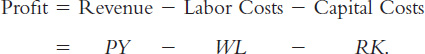
To see how profit depends on the factors of production, we use the production function Y = F(K, L) to substitute for Y to obtain

Profit = PF(K, L) − WL − RK.

This equation shows that profit depends on the product price P, the factor prices W and R, and the factor quantities L and K. The competitive firm takes the product price and the factor prices as given and chooses the amounts of labor and capital that maximize profit.

We now know that our firm will hire labor and rent capital in the quantities that maximize profit. But what are those profit-maximizing quantities? To answer this question, we first consider the quantity of labor and then the quantity of capital.

The Marginal Product of Labor The more labor the firm employs, the more output it produces. The marginal product of labor (MPL) is the extra amount of output the firm gets from one extra unit of labor, holding the amount of capital fixed. We can express this using the production function:

MPL = F(K, L + 1) − F(K, L).

The first term on the right-hand side is the amount of output produced with K units of capital and L + 1 units of labor; the second term is the amount of output produced with K units of capital and L units of labor. This equation states that the marginal product of labor is the difference between the amount of output produced with L + 1 units of labor and the amount produced with only L units of labor.

54

Most production functions have the property of diminishing marginal product: holding the amount of capital fixed, the marginal product of labor decreases as the amount of labor increases. To see why, consider again the production of bread at a bakery. As a bakery hires more labor, it produces more bread. The MPL is the amount of extra bread produced when an extra unit of labor is hired. As more labor is added to a fixed amount of capital, however, the MPL falls. Fewer additional loaves are produced because workers are less productive when the kitchen is more crowded. In other words, holding the size of the kitchen fixed, each additional worker adds fewer loaves of bread to the bakery’s output.

Figure 3-3 graphs the production function. It illustrates what happens to the amount of output when we hold the amount of capital constant and vary the amount of labor. This figure shows that the marginal product of labor is the slope of the production function. As the amount of labor increases, the production function becomes flatter, indicating diminishing marginal product.

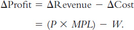
From the Marginal Product of Labor to Labor Demand When the competitive, profit-maximizing firm is deciding whether to hire an additional unit of labor, it considers how that decision would affect profits. It therefore compares the extra revenue from increased production with the extra cost from hiring the additional labor. The increase in revenue from an additional unit of labor depends on two variables: the marginal product of labor and the price of the output. Because an extra unit of labor produces MPL units of output and each unit of output sells for P dollars, the extra revenue is P × MPL. The extra cost of hiring one more unit of labor is the wage W. Thus, the change in profit from hiring an additional unit of labor is

55

The symbol Δ (called delta) denotes the change in a variable.

We can now answer the question we asked at the beginning of this section: how much labor does the firm hire? The firm’s manager knows that if the extra revenue P × MPL exceeds the wage W, an extra unit of labor increases profit. Therefore, the manager continues to hire labor until the next unit would no longer be profitable—that is, until the MPL falls to the point where the extra revenue equals the wage. The competitive firm’s demand for labor is determined by

P × MPL = W.

We can also write this as

MPL = W/P.

W/P is the real wage—the payment to labor measured in units of output rather than in dollars. To maximize profit, the firm hires up to the point at which the marginal product of labor equals the real wage.

For example, again consider a bakery. Suppose the price of bread P is $2 per loaf, and a worker earns a wage W of $20 per hour. The real wage W/P is 10 loaves per hour. In this example, the firm keeps hiring workers as long as the additional worker would produce at least 10 loaves per hour. When the MPL falls to 10 loaves per hour or less, hiring additional workers is no longer profitable.

Figure 3-4 shows how the marginal product of labor depends on the amount of labor employed (holding the firm’s capital stock constant). That is, this figure graphs the MPL schedule. Because the MPL diminishes as the amount of labor increases, this curve slopes downward. For any given real wage, the firm hires up to the point at which the MPL equals the real wage. Hence, the MPL schedule is also the firm’s labor demand curve.

The Marginal Product of Capital and Capital Demand The firm decides how much capital to rent in the same way it decides how much labor to hire. The marginal product of capital (MPK) is the amount of extra output the firm gets from an extra unit of capital, holding the amount of labor constant:

MPK = F(K + 1, L) − F(K, L).

Thus, the marginal product of capital is the difference between the amount of output produced with K + 1 units of capital and that produced with only K units of capital.

Like labor, capital is subject to diminishing marginal product. Once again consider the production of bread at a bakery. The first several ovens installed in the kitchen will be very productive. However, if the bakery installs more and more ovens, while holding its labor force constant, it will eventually contain more ovens than its employees can effectively operate. Hence, the marginal product of the last few ovens is lower than that of the first few.

56

The increase in profit from renting an additional machine is the extra revenue from selling the output of that machine minus the machine’s rental price:

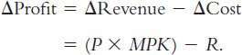
To maximize profit, the firm continues to rent more capital until the MPK falls to equal the real rental price:

MPK = R/P.

The real rental price of capital is the rental price measured in units of goods rather than in dollars.

To sum up, the competitive, profit-maximizing firm follows a simple rule about how much labor to hire and how much capital to rent. The firm demands each factor of production until that factor’s marginal product falls to equal its real factor price.

Having analyzed how a firm decides how much of each factor to employ, we can now explain how the markets for the factors of production distribute the economy’s total income. If all firms in the economy are competitive and profit maximizing, then each factor of production is paid its marginal contribution to the production process. The real wage paid to each worker equals the MPL, and the real rental price paid to each owner of capital equals the MPK. The total real wages paid to labor are therefore MPL × L, and the total real return paid to capital owners is MPK × K.

57

The income that remains after the firms have paid the factors of production is the economic profit of the owners of the firms:

Economic Profit = Y − (MPL × L) − (MPK × K).

Note that income Y and economic profit are here being expressed in real terms—that is, in units of output rather than in dollars. Because we want to examine the distribution of income, we rearrange the terms as follows:

Y = (MPL × L) + (MPK × K) + Economic Profit.

Total income is divided among the return to labor, the return to capital, and economic profit.

How large is economic profit? The answer is surprising: if the production function has the property of constant returns to scale, as is often thought to be the case, then economic profit must be zero. That is, nothing is left after the factors of production are paid. This conclusion follows from a famous mathematical result called Euler’s theorem,2 which states that if the production function has constant returns to scale, then

F(K, L) = (MPK × K) + (MPL × L).

If each factor of production is paid its marginal product, then the sum of these factor payments equals total output. In other words, constant returns to scale, profit maximization, and competition together imply that economic profit is zero.

If economic profit is zero, how can we explain the existence of “profit” in the economy? The answer is that the term “profit” as normally used is different from economic profit. We have been assuming that there are three types of agents: workers, owners of capital, and owners of firms. Total income is divided among wages, return to capital, and economic profit. In the real world, however, most firms own rather than rent the capital they use. Because firm owners and capital owners are the same people, economic profit and the return to capital are often lumped together. If we call this alternative definition accounting profit, we can say that

Accounting Profit = Economic Profit + (MPK × K).

Under our assumptions—constant returns to scale, profit maximization, and competition—economic profit is zero. If these assumptions approximately describe the world, then the “profit” in the national income accounts must be mostly the return to capital.

58

We can now answer the question posed at the beginning of this chapter about how the income of the economy is distributed from firms to households. Each factor of production is paid its marginal product, and these factor payments exhaust total output. Total output is divided between the payments to capital and the payments to labor, depending on their marginal productivities.

What production function describes how actual economies turn capital and labor into GDP? One answer to this question came from a historic collaboration between a U.S. senator and a mathematician.

Paul Douglas was a U.S. senator from Illinois from 1949 to 1967. In 1927, however, when he was still a professor of economics, he noticed a surprising fact: the division of national income between capital and labor had been roughly constant over a long period. In other words, as the economy grew more prosperous over time, the total income of workers and the total income of capital owners grew at almost exactly the same rate. This observation caused Douglas to wonder what conditions might lead to constant factor shares.

59

Douglas asked Charles Cobb, a mathematician, what production function, if any, would produce constant factor shares if factors always earned their marginal products. The production function would need to have the property that

Capital Income = MPK × K = αY

and

Labor Income = MPL × L = (1 − α) Y,

where α is a constant between zero and one that measures capital’s share of income. That is, α determines what share of income goes to capital and what share goes to labor. Cobb showed that the function with this property is

F(K,L) = A K^αL^1−α,

where A is a parameter greater than zero that measures the productivity of the available technology. This function became known as the Cobb-Douglas production function.

Let’s take a closer look at some of the properties of this production function. First, the Cobb–Douglas production function has constant returns to scale. That is, if capital and labor are increased by the same proportion, then output increases by that proportion as well.4

Next, consider the marginal products for the Cobb–Douglas production function. The marginal product of labor is5

MPL = (1 − α) A K^αL^−α,

60

and the marginal product of capital is

MPK = α A K^α−1L^1−α.

From these equations, recalling that α is between zero and one, we can see what causes the marginal products of the two factors to change. An increase in the amount of capital raises the MPL and reduces the MPK. Similarly, an increase in the amount of labor reduces the MPL and raises the MPK. A technological advance that increases the parameter A raises the marginal product of both factors proportionately.

The marginal products for the Cobb–Douglas production function can also be written as6

MPL = (1 − α) Y/L.

MPL = αY/K.

The MPL is proportional to output per worker, and the MPK is proportional to output per unit of capital. Y/L is called average labor productivity, and Y/K is called average capital productivity. If the production function is Cobb–Douglas, then the marginal productivity of a factor is proportional to its average productivity.

We can now verify that if factors earn their marginal products, then the parameter α indeed tells us how much income goes to labor and how much goes to capital. The total amount paid to labor, which we have seen is MPL × L, equals (1 − α)Y. Therefore, (1 − α) is labor’s share of output. Similarly, the total amount paid to capital, MPK × K, equals αY, and α is capital’s share of output. The ratio of labor income to capital income is a constant, (1 − α)/α, just as Douglas observed. The factor shares depend only on the parameter α, not on the amounts of capital or labor or on the state of technology as measured by the parameter A.

More recent U.S. data are also consistent with the Cobb–Douglas production function. Figure 3-5 shows the ratio of labor income to total income in the United States from 1960 to 2013. Despite the many changes in the economy over the past five decades, this ratio has remained about 2/3. This division of income is easily explained by a Cobb–Douglas production function in which the parameter α is about 1/3. According to this parameter, capital receives a third of income, and labor receives two-thirds.

Although the capital and labor shares are approximately constant, they are not exactly constant. In particular, Figure 3-5 shows that the labor share fell from a high of 72 percent in 1970 to 63 percent in 2013. The flip side, of course, is that the capital share increased during this period from 28 percent to 37 percent. The reason for this change in factor shares is not well understood. One possibility is that technological progress over the past several decades has not simply increased the parameter A but may have also changed the relative importance of capital and labor in the production process, thereby altering the parameter α as well. But it is also possible that there are important determinants of incomes that are not well captured by the Cobb–Douglas production function together with the competitive model of factor markets.7

61

The Cobb–Douglas production function is not the last word in explaining the economy’s production of goods and services or the distribution of national income between capital and labor. It is, however, a good place to start.

62

One striking development about the U.S. economy, as well as many other economies around the world, is an increase in income inequality over the past several decades. Figure 3-6 illustrates this phenomenon by showing the Gini coefficient for family incomes from 1947 to 2012. The Gini coefficient is a measure of income dispersion: it is between zero and one, with zero representing perfect equality (all families have the same income) and one representing perfect inequality (all income goes to one family).8 The figure shows that the Gini coefficient fell from 0.38 in 1947 to a low of 0.35 in 1968, a period when incomes were becoming slightly more equal. But the economy then entered a period of rising inequality. The Gini coefficient rose to 0.45 in 2012.

64

What explains increasing inequality in family incomes? Part of the story is the change in factor shares discussed earlier. Because capital income tends to be more concentrated in higher-income households than is labor income, a fall in the labor share and rise in the capital share tends to increase inequality. But the change in factor shares is only a small piece of the puzzle. More important, if we look within labor income, we find that the gap between the earnings of high-wage workers and the earnings of low-wage workers has grown substantially since the 1970s.

Economists have spent much research effort trying to explain increasing inequality of labor earnings. As yet no definitive conclusion has emerged, but a prominent diagnosis comes from economists Claudia Goldin and Lawrence Katz in their book The Race Between Education and Technology.9 Their bottom line is that “the sharp rise in inequality was largely due to an educational slowdown.”

According to Goldin and Katz, for the past century technological progress has been a steady economic force, not only increasing average living standards but also increasing the demand for skilled workers relative to unskilled workers. Skilled workers are needed to apply and manage new technologies, while less skilled workers are more likely to become obsolete. By itself, this skill-biased technological change tends to raise the wages of skilled workers relative to the wages of unskilled workers, thereby increasing inequality.

For much of the twentieth century, however, skill-biased technological change was outpaced by advances in educational attainment. In other words, while technological progress increased the demand for skilled workers, our educational system increased the supply of skilled workers even faster. As a result, skilled workers did not benefit disproportionately from economic growth. Indeed, until the 1970s, wages for the skilled workers grew more slowly than wages for unskilled workers, reducing inequality.

Recently things have changed. Over the last several decades, technological progress kept up its pace, but educational advancement slowed down. Numbers from Goldin and Katz show the magnitude of what happened. The cohort of workers born in 1950 averaged 4.67 more years of schooling than the cohort born in 1900, representing an increase of 0.93 years of schooling in each decade. By contrast, the cohort born in 1975 had only 0.74 more years of schooling than that born in 1950, an increase of only 0.30 years per decade. That is, the pace of educational advancement fell by 68 percent.

Because growth in the supply of skilled workers has slowed, their wages have grown relative to those of the unskilled. This phenomenon is evident in Goldin and Katz’s estimates of the financial return to education. In 1980, each year of college raised a person’s wage by 7.6 percent. In 2005, each year of college yielded an additional 12.9 percent. Over this time period, the rate of return from each year of graduate school rose even more—from 7.3 to 14.2 percent. (Implication for personal decisionmaking: for most people, college and graduate school are investments well worth making.)

65

Increasing income inequality has become a prominent topic in the debate over public policy. In response to these economic developments, some policymakers advocate a more redistributive system of taxes and transfers, to take from those higher on the economic ladder and give to those on the lower rungs. Such an approach treats the symptoms but not the underlying causes of rising inequality. If the conclusions of Goldin and Katz are correct, reversing the rise in income inequality will likely require putting more of society’s resources into education (which economists call human capital). Educational reform is a topic beyond the scope of this book, but it is worth noting that, if successful, such reform could have profound effects on the economy and the distribution of income.