6.2 Saving and Investment in a Small Open Economy
So far in our discussion of the international flows of goods and capital, we have rearranged accounting identities. That is, we have defined some of the variables that measure transactions in an open economy, and we have shown the links among these variables that follow from their definitions. Our next step is to develop a model that explains the behavior of these variables. We can then use the model to answer questions such as how the trade balance responds to changes in policy.
146
Capital Mobility and the World Interest Rate
In a moment we present a model of the international flows of capital and goods. Because the trade balance equals the net capital outflow, which in turn equals saving minus investment, our model focuses on saving and investment. To develop this model, we use some elements that should be familiar from Chapter 3, but unlike with the Chapter 3 model, we do not assume that the real interest rate equilibrates saving and investment. Instead, we allow the economy to run a trade deficit and borrow from other countries or to run a trade surplus and lend to other countries.
If the real interest rate does not adjust to equilibrate saving and investment in this model, what does determine the real interest rate? We answer this question here by considering the simple case of a small open economy with perfect capital mobility. By “small” we mean that this economy is a small part of the world market and thus, by itself, can have only a negligible effect on the world interest rate. By “perfect capital mobility” we mean that residents of the country have full access to world financial markets. In particular, the government does not impede international borrowing or lending.
Because of this assumption of perfect capital mobility, the interest rate in our small open economy, r, must equal the world interest rate r*, the real interest rate prevailing in world financial markets:
r = r*.
Residents of the small open economy need never borrow at any interest rate above r*, because they can always get a loan at r* from abroad. Similarly, residents of this economy need never lend at any interest rate below r*, because they can always earn r* by lending abroad. Thus, the world interest rate determines the interest rate in our small open economy.
Let’s briefly discuss what determines the world real interest rate. In a closed economy, the equilibrium of domestic saving and domestic investment determines the interest rate. Barring interplanetary trade, the world economy is a closed economy. Therefore, the equilibrium of world saving and world investment determines the world interest rate. Our small open economy has a negligible effect on the world real interest rate because, being a small part of the world, it has a negligible effect on world saving and world investment. Hence, our small open economy takes the world interest rate as exogenously given.
Why Assume a Small Open Economy?
The analysis in the body of this chapter assumes that the nation being studied is a small open economy. (The same approach is taken in Chapter 13, which examines short-
Q: Is the United States well described by the assumption of a small open economy?
A: No, it is not, at least not completely. The United States does borrow and lend in world financial markets, and these markets exert a strong influence over the U.S. real interest rate, but it would be an exaggeration to say that the U.S. real interest rate is determined solely by world financial markets.
147
Q: So why are we assuming a small open economy?
A: Some nations, such as Canada and the Netherlands, are better described by the assumption of a small open economy. Yet the main reason for making this assumption is to develop understanding and intuition for the macroeconomics of open economies. Remember from Chapter 1 that economic models are built with simplifying assumptions. An assumption need not be realistic to be useful. Assuming a small open economy simplifies the analysis greatly and, therefore, helps clarify our thinking.
Q: Can we relax this assumption and make the model more realistic?
A: Yes, we can, and we will. The appendix to this chapter (and the appendix to Chapter 13) considers the more realistic and more complicated case of a large open economy. Some instructors skip directly to this material when teaching these topics because the approach is more realistic for economies such as that of the United States. Others think that students should walk before they run and, therefore, begin with the simplifying assumption of a small open economy.
The Model
To build the model of the small open economy, we take three assumptions from Chapter 3:
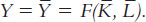
The economy’s output Y is fixed by the factors of production and the production function. We write this as
Consumption C is positively related to disposable income Y – T.
We write the consumption function as
C = C(Y – T).
Investment I is negatively related to the real interest rate r. We write the investment function as
I = I(r).
These are the three key parts of our model. If you do not understand these relationships, review Chapter 3 before continuing.
We can now return to the accounting identity and write it as
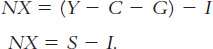
Substituting the Chapter 3 assumptions recapped above and the assumption that the interest rate equals the world interest rate, we obtain
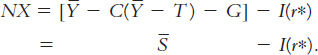
148
This equation shows that the trade balance NX depends on those variables that determine saving S and investment I. Because saving depends on fiscal policy (lower government purchases G or higher taxes T raise national saving) and investment depends on the world real interest rate r* (a higher interest rate makes some investment projects unprofitable), the trade balance depends on these variables as well.
In Chapter 3 we graphed saving and investment as in Figure 6-2. In the closed economy studied in that chapter, the real interest rate adjusts to equilibrate saving and investment—

At this point, you might wonder about the mechanism that causes the trade balance to equal the net capital outflow. The determinants of the capital flows are easy to understand. When saving falls short of investment, investors borrow from abroad; when saving exceeds investment, the excess is lent to other countries. But what causes those who import and export to behave so that the international flow of goods exactly balances this international flow of capital? For now we leave this question unanswered, but we return to it in Section 6-3 when we discuss the determination of exchange rates.
How Policies Influence the Trade Balance
Suppose that the economy begins in a position of balanced trade. That is, at the world interest rate, investment I equals saving S, and net exports NX equal zero. Let’s use our model to predict the effects of government policies at home and abroad.
149
Fiscal Policy at Home Consider first what happens to the small open economy if the government expands domestic spending by increasing government purchases. The increase in G reduces national saving, because S = Y – C – G. With an unchanged world real interest rate, investment remains the same. Therefore, saving falls below investment, and some investment must now be financed by borrowing from abroad. Because NX = S – I, the fall in S implies a fall in NX. The economy now runs a trade deficit.
The same logic applies to a decrease in taxes. A tax cut lowers T, raises disposable income Y – T, stimulates consumption, and reduces national saving. (Even though some of the tax cut finds its way into private saving, public saving falls by the full amount of the tax cut; in total, saving falls.) Because NX = S – I, the reduction in national saving in turn lowers NX.
Figure 6-3 illustrates these effects. A fiscal policy change that increases private consumption C or public consumption G reduces national saving (Y – C – G) and, therefore, shifts the vertical line that represents saving from S1 to S2. Because NX is the distance between the saving schedule and the investment schedule at the world interest rate, this shift reduces NX. Hence, starting from balanced trade, a change in fiscal policy that reduces national saving leads to a trade deficit.

Fiscal Policy Abroad Consider now what happens to a small open economy when foreign governments increase their government purchases. If these foreign countries are a small part of the world economy, then their fiscal change has a negligible impact on other countries. But if these foreign countries are a large part of the world economy, their increase in government purchases reduces world saving. The decrease in world saving causes the world interest rate to rise, just as we saw in our closed-
The increase in the world interest rate raises the cost of borrowing and, thus, reduces investment in our small open economy. Because there has been no change in domestic saving, saving S now exceeds investment I, and some of our saving begins to flow abroad. Because NX = S – I, the reduction in I must also increase NX. Hence, reduced saving abroad leads to a trade surplus at home.
150
Figure 6-4 illustrates how a small open economy starting from balanced trade responds to a foreign fiscal expansion. Because the policy change occurs abroad, the domestic saving and investment schedules remain the same. The only change is an increase in the world interest rate from  to
to  . The trade balance is the difference between the saving and investment schedules; because saving exceeds investment at
, there is a trade surplus. Hence, starting from balanced trade, an increase in the world interest rate due to a fiscal expansion abroad leads to a trade surplus.
. The trade balance is the difference between the saving and investment schedules; because saving exceeds investment at
, there is a trade surplus. Hence, starting from balanced trade, an increase in the world interest rate due to a fiscal expansion abroad leads to a trade surplus.

Shifts in Investment Demand Consider what happens to our small open economy if its investment schedule shifts outward—

Evaluating Economic Policy
Our model of the open economy shows that the flow of goods and services measured by the trade balance is inextricably connected to the international flow of funds for capital accumulation. The net capital outflow is the difference between domestic saving and domestic investment. Thus, the impact of economic policies on the trade balance can always be found by examining their impact on domestic saving and domestic investment. Policies that increase investment or decrease saving tend to cause a trade deficit, and policies that decrease investment or increase saving tend to cause a trade surplus.
151
Our analysis of the open economy has been positive, not normative. That is, our analysis of how economic policies influence the international flows of capital and goods has not told us whether these policies are desirable. Evaluating economic policies and their impact on the open economy is a frequent topic of debate among economists and policymakers.
When a country runs a trade deficit, policymakers must confront the question of whether it represents a national problem. Most economists view a trade deficit not as a problem in itself, but perhaps as a symptom of a problem. A trade deficit could be a reflection of low saving. In a closed economy, low saving leads to low investment and a smaller future capital stock. In an open economy, low saving leads to a trade deficit and a growing foreign debt, which eventually must be repaid. In both cases, high current consumption leads to lower future consumption, implying that future generations bear the burden of low national saving.
Yet trade deficits are not always a reflection of an economic malady. When poor rural economies develop into modern industrial economies, they sometimes finance their high levels of investment with foreign borrowing. In these cases, trade deficits are a sign of economic development. For example, South Korea ran large trade deficits throughout the 1970s and early 1980s, and it became one of the success stories of economic growth. The lesson is that one cannot judge economic performance from the trade balance alone. Instead, one must look at the underlying causes of the international flows.
152
CASE STUDY
The U.S. Trade Deficit
During the 1980s, 1990s, and 2000s, the United States ran large trade deficits. Panel (a) of Figure 6-6 documents this experience by showing net exports as a percentage of GDP. The exact size of the trade deficit fluctuated over time, but it was large throughout these three decades. In 2013, the trade deficit was $497 billion, or 3.0 percent of GDP. As accounting identities require, this trade deficit had to be financed by borrowing from abroad (or, equivalently, by selling U.S. assets abroad). During this period, the United States went from being the world’s largest creditor to the world’s largest debtor.

What caused the U.S. trade deficit? There is no single explanation. But to understand some of the forces at work, it helps to look at national saving and domestic investment, as shown in panel (b) of the figure. Keep in mind that the trade deficit is the difference between saving and investment.
The start of the trade deficit coincided with a fall in national saving. This development can be explained by the expansionary fiscal policy in the 1980s. With the support of President Reagan, the U.S. Congress passed legislation in 1981 that substantially cut personal income taxes over the next three years. Because these tax cuts were not met with equal cuts in government spending, the federal budget went into deficit. These budget deficits were among the largest ever experienced in a period of peace and prosperity, and they continued long after Reagan left office. According to our model, such a policy should reduce national saving, thereby causing a trade deficit. And, in fact, that is exactly what happened. Because the government budget and trade balance went into deficit at roughly the same time, these shortfalls were called the twin deficits.
Things started to change in the 1990s, when the U.S. federal government got its fiscal house in order. The first President Bush and President Clinton both signed tax increases, while Congress kept a lid on spending. In addition to these policy changes, rapid productivity growth in the late 1990s raised incomes and, thus, further increased tax revenue. These developments moved the U.S. federal budget from deficit to surplus, which in turn caused national saving to rise.
In contrast to our model’s predictions, the increase in national saving did not coincide with a shrinking trade deficit, because domestic investment rose at the same time. The likely explanation is that the boom in information technology caused an expansionary shift in the U.S. investment function. Even though fiscal policy was pushing the trade deficit toward surplus, the investment boom was an even stronger force pushing the trade balance toward deficit.
In the early 2000s, fiscal policy once again put downward pressure on national saving. With the second President Bush in the White House, tax cuts were signed into law in 2001 and 2003, while the war on terror led to substantial increases in government spending. The federal government was again running budget deficits. National saving fell to historic lows, and the trade deficit reached historic highs.
A few years later, the trade deficit started to shrink somewhat, as the economy experienced a substantial decline in housing prices (a phenomenon examined in Case Studies in Chapter 12 and Chapter 17). Lower housing prices led to a substantial decline in residential investment. The trade deficit fell from 5.5 percent of GDP at its peak in 2006 to 3.0 percent in 2013.
153
154
The history of the U.S. trade deficit shows that this statistic, by itself, does not tell us much about what is happening in the economy. We have to look deeper at saving, investment, and the policies and events that cause them (and thus the trade balance) to change over time.1 
CASE STUDY
Why Doesn't Capital Flow to Poor Countries?
The U.S. trade deficit discussed in the previous Case Study represents a flow of capital into the United States from the rest of the world. What countries were the source of these capital flows? Because the world is a closed economy, the capital must have been coming from those countries that were running trade surpluses. In 2013, this group included many nations that were far poorer than the United States, such as China, Nigeria, Venezuela, and Vietnam. In these nations, saving exceeded investment in domestic capital. These countries were sending funds abroad to countries like the United States, where investment in domestic capital exceeded saving.
From one perspective, the direction of international capital flows is a paradox. Recall our discussion of production functions in Chapter 3. There, we established that an empirically realistic production function is the Cobb–
F(K, L) = A KαL1–
where K is capital, L is labor, A is a variable representing the state of technology, and α is a parameter that determines capital’s share of total income. For this production function, the marginal product of capital is
MPK = αA(K/L)α–1.
The marginal product of capital tells us how much extra output an extra unit of capital would produce. Because α is capital’s share, it must be less than 1, so α – 1 < 0. This means that an increase in K/L decreases MPK. In other words, holding other variables constant, the more capital a nation has, the less valuable an extra unit of capital is. This phenomenon of diminishing marginal product says that capital should be more valuable where capital is scarce.
This prediction, however, seems at odds with the international flow of capital represented by trade imbalances. Capital does not seem to flow to those nations where it should be most valuable. Instead of capital-
One reason is that there are important differences among nations other than their accumulation of capital. Poor nations have not only lower levels of capital accumulation per worker (represented by K/L) but also inferior production capabilities (represented by the variable A). For example, compared to rich nations, poor nations may have less access to advanced technologies, lower levels of education (or human capital), or less efficient economic policies. Such differences could mean less output for given inputs of capital and labor; in the Cobb–
155
A second reason capital might not flow to poor nations is that property rights are often not enforced. Corruption is much more prevalent; revolutions, coups, and expropriation of wealth are more common; and governments often default on their debts. So even if capital is more valuable in poor nations, foreigners may avoid investing their wealth there simply because they are afraid of losing it. Moreover, local investors face similar incentives. Imagine that you live in a poor nation and are lucky enough to have some wealth to invest; you might well decide that putting it in a safe country like the United States is your best option, even if capital is less valuable there than in your home country.
Whichever of these two reasons is correct, the challenge for poor nations is to find ways to reverse the situation. If these nations offered the same production efficiency and legal protections as the U.S. economy, the direction of international capital flows would likely reverse. The U.S. trade deficit would become a trade surplus, and capital would flow to these emerging nations. Such a change would help the poor of the world escape poverty.2